research · 2026-10-08 · revised 2026-10-11 · 43 min read
Certified patch skipping for fixed-camera video
What can be proved about the patches a video model never sees, and how far that proof stretches on real cameras.
Continued
There is a second part: Certified skipping, part 2: the picture the model holds. It finds that the certificate below is about a re-levelled image and not about the copy a model holds, closes that with a one-line change, and tests it on real sunset footage.
the idea in three clips
Abstract
Video language models spend most of their tokens on patches that have not changed. The rules used today to skip those patches are heuristics: they compare the mean of a patch between consecutive frames and say nothing about what was thrown away. This note starts from a rule that fits on one line, drop a patch when the spread of its change is below , and proves what that buys: by stability of persistence diagrams, no object of contrast can appear, vanish, split or merge inside a dropped patch, and the threshold cannot be raised without losing that statement.
On real cameras the rule drops 99 % of patches on clean codecs and only 73 % on a noisy analog hallway. The cause is sub-pixel edge jitter, and it motivates three further certificates built from different mathematics: transport (the flat norm), multi-scale box averages, and a quotient by sub-pixel motion. Quotient plus multi-scale keeps 2.7 to 5.5 % of patches where the original rule keeps 15 to 19 %, at the same 100 % recall of the planted small and slow-fading objects. A sequential layer taken from quickest change detection then catches persistent objects an order of magnitude fainter than any single-frame rule can see: across 25 fixed-camera clips, recall of contrast-12 objects goes from 0.13 to 0.96 for at most 0.3 points of drop rate. The median drop rate over those clips is 0.989, at an operating point whose worst-case certificate is weaker than the one-line rule's: contrast 80 for a single pixel, falling to 30 for an object that contains a 7×7 box. The one-line rule at has a median of 0.956.
The same machinery gives class-agnostic, pixel-level object masks at 18 to 29 fps on 1080p and 140 to 178 fps at CIF resolution on a laptop CPU, with a certificate for the labels that are reused. The masks are not scored against human-labelled ground truth. One idea did not work, and the note says so: adaptive look scheduling is sound but does not beat uniform sampling, for a structural reason. End to end with an unmodified Qwen2-VL-2B and every rule at the same drop rate, an object that fades in slowly reaches the model's answer in 23 of 26 perceivable cases through the certified rule and in 2 of 26 through a consecutive-frame rule. That test shows the model an image rebuilt from each rule's decisions. It does not skip tokens inside the model.
1The problem
A vision transformer cuts each frame into patches, typically 16×16 pixels, and turns every patch into a token. A fixed camera at 1080p produces about eight thousand patches per frame, and almost all of them are the same wall, floor and sky as a second ago. If the model already holds a token for a patch and the patch has not changed, the token can be reused and the patch need not be processed again.
Everything depends on what "has not changed" means. The rules in use, in systems such as EVS, TimeChat-style streaming models and run-length tokenisation [16], compare the mean absolute difference of a patch between consecutive frames against a threshold. That is cheap and usually fine. It has two blind spots, and no statement of what it guarantees:
- A change that is slow enough never exceeds the per-frame threshold, however large it eventually becomes.
- A change that is small in area is averaged away over the 256 pixels of the patch.
The question this project asks is different from "which heuristic drops more". It is: can a skip rule come with a theorem that names what cannot have happened in a patch the model did not look at, and is such a rule usable on real cameras?
Setting. A fixed camera produces grey frames. A patch of pixels has a reference , the last copy that was sent to the model, and a new value . Write . A skip rule is a statistic and a threshold. A certificate is a theorem of the form: if , then nothing of the following kind happened in . Unless stated otherwise and intensities are 8-bit grey levels.
Note the comparison is always against the last kept copy and never against the previous frame. That one choice already removes the slow-change blind spot: change accumulates in until it is large enough to be kept.
2The range rule
2.1Statement
Rule 1 (range).
With on the patch,
and otherwise keep the patch and set . On a dropped patch the model's view is the reference shifted by the midrange of the change,
The statistic is the spread of the change, not its size. A uniform brightness change has spread zero and is dropped, which is right: nothing appeared or disappeared, and the view compensates for it through .
2.2What "an object" means here
The guarantee is stated in the language of persistent homology, because that is the mathematics in which "an object of contrast " has a precise meaning that does not depend on shape.
For a function on the patch, sweep a threshold upward and watch the sublevel set . A dark blob is born when passes a local minimum and dies when its component merges into an older one. Its persistence, death minus birth, is exactly the contrast of the blob against its surroundings. The multiset of (birth, death) pairs is the persistence diagram . Superlevel sets give bright blobs in the same way. The essential class is capped at the patch extremum, so a flat patch has no features and a single blob has contrast equal to its depth.
Two diagrams are compared with the bottleneck distance : the smallest such that the features can be matched to each other, or to nothing, with every match moving a point by at most and every unmatched feature having persistence at most . The one theorem everything rests on is stability [1]:
2.3Guarantee
Theorem 1 (range certificate).
If a patch is dropped by Rule 1, then
- : the view is pointwise within of the truth;
- , for dark blobs and for bright blobs;
- every feature's contrast changes by at most , and no feature of contrast is born from nothing or dies into nothing while the patch is dropped.
Proof.
Let and . For every pixel, , and both ends are attained, which is (1). Stability applied to and gives (2). Adding the constant shifts every birth and death of by and leaves persistences unchanged, so has the features of . In a matching of cost at most a matched feature's birth and death each move by at most , so its persistence changes by at most . A feature left unmatched has persistence at most . So a feature of contrast in is matched to a feature of , and conversely, which is (3).
2.4Tightness
Proposition 2 (the threshold cannot be moved).
For every change pattern with there is a scene in which that change creates an object of contrast exactly . Hence no rule that looks only at the change can drop at spread and keep the guarantee of Theorem 1.
Proof.
Take flat. Then has no features, and has , so its deepest minimum is a dark blob of persistence .
2.5Noise sets the usable threshold
For independent noise of standard deviation per frame, the expected spread over the pixels of a static patch is about . The threshold must therefore sit well above , and a Gaussian model gives a ceiling on the achievable drop rate for each . This ceiling is the first thing to compare with real footage, and Section 3 shows it is the wrong model.
2.6What the rule does not cover
- Camera motion. The certificate is per patch for a fixed camera.
- Features finer than one patch's topology, and anything that straddles patches in a way no single patch sees as a change.
- A change that is uniform over a whole patch. The flat interior of an object larger than a patch shifts each patch it covers by a constant, which has spread zero. Those patches are dropped and the change is carried only by the shift . The view adds back. A model that reuses a cached token would have to be sent and be able to apply it.
- Rings. The theorem covers as well, but the checker used for audits computes only (dark and bright blobs).
Details of the semantics: the first frame is always kept and excluded from the drop rate; pixels beyond the last full patch row or column are ignored; 8-bit input is differenced in 32-bit integers; the comparison with is strict.
3First experiments
All numbers come from the scripts of the reference implementation (C++ core, numpy reference, Section 14) on an Apple M4, with and grey levels unless stated.
3.1Real footage
Sources: the Xiph.org derf test set (uncompressed CIF, 30 fps; hall_monitor is a fixed hallway camera with two people walking, akiyo a news anchor on a static backdrop), the Blender Foundation film Tears of Steel (CC-BY, live action with cuts and camera motion, 720p H.264, 12 minutes), the VIRAT public release (parking lots and streets) and the CAVIAR lobby and corridor cameras.
Table 1. Drop rate of the range rule against threshold. The Gaussian ceiling is what independent sensor noise of the measured would allow at .
| clip | camera | ceiling @32 | |||||
|---|---|---|---|---|---|---|---|
| hall_monitor | fixed, analog-era CCTV | 1.7 | 0.26 | 0.61 | 0.73 | 0.87 | 1.00 |
| akiyo | fixed, clean digital | 0.0 | 0.82 | 0.87 | 0.89 | 0.92 | 1.00 |
| Tears of Steel, 2 fps | moving, cuts | 1.9 | 0.25 | 0.31 | 0.37 | 0.46 | 1.00 |
| Tears of Steel, 24 fps | moving, cuts | 0.58 | |||||
| VIRAT 000200_00, 10 fps | parking lot, 720p MPEG-4 | 0.97 | 0.99 | 0.99 | 0.99 | ||
| VIRAT 000200_01, 10 fps | same camera | 0.95 | 0.98 | 0.98 | 0.99 | ||
| CAVIAR WalkByShop1cor | mall corridor, MPEG-1 | 0.83 | 0.90 | 0.93 | 0.95 | ||
| CAVIAR LeftBag | lobby, several people | 0.35 | 0.59 | 0.77 | 0.90 | ||
| CAVIAR Walk1 | lobby | 0.36 | 0.61 | 0.78 | 0.90 | ||
| CAVIAR Meet_Crowd | lobby | 0.37 | 0.61 | 0.77 | 0.89 |
The for Tears of Steel is inflated by motion: the robust estimator assumes half the patches are static.
Soundness. 500 + 500 + 300 dropped patches were audited with exact bottleneck distances, dark and bright blobs. There were 0 violations, and the worst ratio of bottleneck distance to was 1.000: the bound is attained and never exceeded.
Throughput. The C++ core processed the full film, 17,620 frames at 1280×534 with decoding included, at 836 frames per second (571 megapixels per second), and about 1,150 frames per second on 1080p synthetic input.
3.2Synthetic benchmark at matched budgets
Three static scenes, 40 s at 2 fps, 640×360, H.264 at crf 23, sensor noise before encoding. The certified rule runs at and dropped 0.99 to 1.00. Every baseline is calibrated on an object-free control clip to drop , so the baselines always have at least as much keep budget as the certified rule.
Table 2. Objects caught out of 192 planted, at matched drop budgets, and the worst error of the model's view.
| rule | 5×5 px, one frame, contrast 48 | 8×8 px fading in over 8 s to 64 | worst view error (grey) |
|---|---|---|---|
| certified, | 192 / 192 | 192 / 192 | 15.5 (proved) |
| consecutive-frame mean | 192 / 192 | 168 / 192 | not bounded |
| mean against last kept | 192 / 192 | 192 / 192 | 46 (measured) |
| uniform sampling | 4 / 192 | 45 / 192 | not bounded |
In a harder setting (crf 18, , global flicker of ) the certified rule again caught 192 and 192; the consecutive-frame mean caught 192 and 53; mean against last kept caught 192 and 192 with a measured worst error of 30; uniform sampling caught 2 and 49.
For objects below the averaging threshold (3×3 px, contrast 40, so a mean contribution of against a calibrated threshold near 2.5): certified 192, consecutive mean 184, mean against last kept 187, uniform 5.
A soundness audit of 2,000 dropped synthetic patches found 0 violations, worst ratio 0.875.
3.3What the footage said
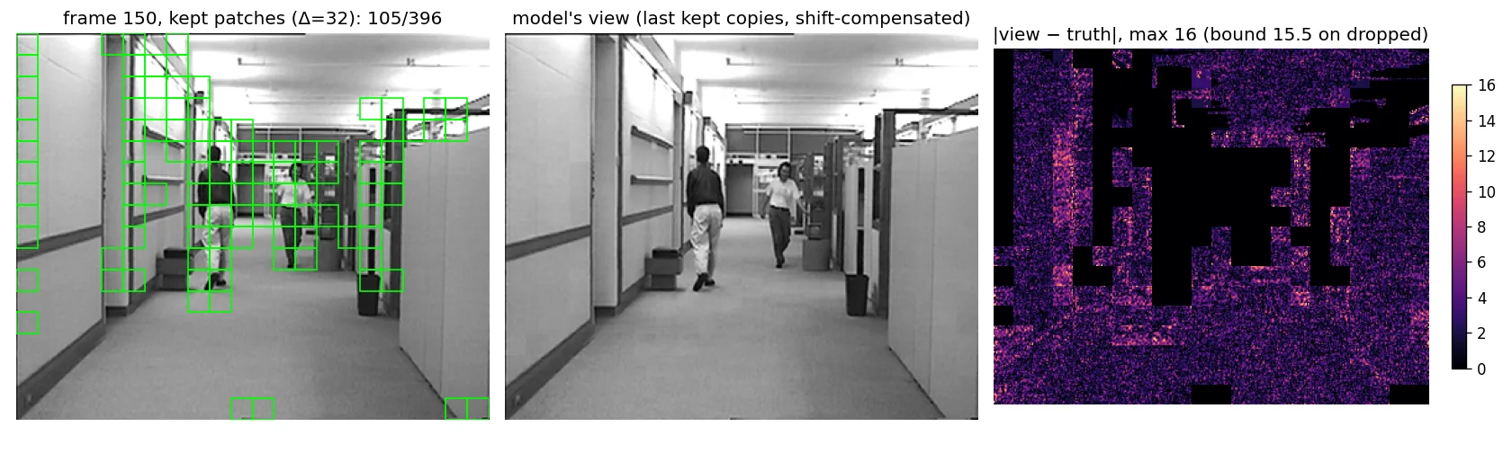
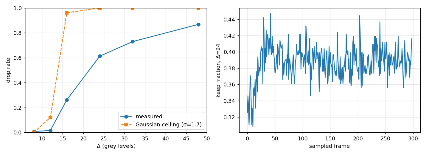
Four findings came out of this first round.
- A clean static camera is close to the synthetic ideal: 89 % on akiyo, 98 to 99 % on VIRAT, where the MPEG-4 encoder has already zeroed static macroblocks and almost all of the kept budget goes to moving people and cars.
- A noisy static camera is not: 73 % on the hallway, where the Gaussian model predicts about 100 %. The shortfall is not sensor noise. Figure 1 shows what is being kept: strips along wall edges. A sub-pixel jiggle of a high-contrast edge changes a one-pixel column by the full contrast of the edge, and is maximally sensitive to exactly that. This is the real-footage cost of the guarantee.
- Cinematic footage is out of scope: 37 % at 2 fps and 58 % at 24 fps, with 30-second windows ranging from 11 % to 64 %. That confirms the fixed-camera caveat; it does not extend the claim.
- The baselines fail on slow change, not on small objects, at realistic sizes. The small-object blind spot of averaging rules appears only when area × contrast / falls below their threshold. Mean against last kept catches everything in these tests, but its view error is unbounded in principle and was measured at two to three times the certified bound.
The claim the data supports is therefore the same drop budget, the same or better recall, and a proved error bound the others lack. It is not the others miss objects.
4Which norm is the right currency
Every skip statistic is a norm of the change, and the choice of norm is the whole story.
Table 3. What each norm of certifies, and what it pays for the two things real cameras do: noise, and a step edge of contrast jittering by pixels.
| norm of | certifies | cost of i.i.d. noise | cost of edge jitter |
|---|---|---|---|
| (range) | every object of contrast , any size | full contrast, on a 1-px strip | |
| / mean | objects of mass (area × contrast) | × area | × edge length |
| flat norm (transport) | mass created, destroyed or moved further than | between the two | same as |
| multi-scale box max | objects containing a -box, contrast | ||
| after quotienting translations | objects of contrast , up to a sub-pixel move | interpolation error only |
A jittering edge is a real change of real mass. No norm of alone makes it small. Two things do: dilution by area (multi-scale) and explanation by motion (quotient). Transport does not, and the next section says so.
5Transport certificate: the flat norm
Definition (flat norm at scale ).
For a signed mass on the pixel grid and a scale ,
Mass may be moved along grid edges at cost ( distance) per unit, or created and destroyed at cost 1 per unit. By Kantorovich–Rubinstein duality, which is exact here because the problem is a finite linear program,
Rule. With and , drop iff , where is the quadtree bound described below.
Theorem 3 (conservation).
If then for every region , with ,
Proof.
is bounded by 1 and -Lipschitz in the metric, so it is feasible for the dual.
Reading. is the net mass change in plus a tapered ring of width . An object of area and contrast that appears contributes to it, and the only way to stay under is an opposite change of mass at least within pixels. So nothing of mass is created or destroyed. Mass that moves by costs , so motion of at least pixels by mass at least is always kept.
Theorem 4 (linear front ends).
For any filter on ,
Proof.
is dual-feasible.
A ViT patch embedding is a linear map with rows , so on a dropped patch the embedding moves by at most , with the constant computed from the weights.
Tightness. on a flat patch, far from the boundary and with the mean removed, has up to the cost of spreading the compensating mean. A threshold cannot be raised without admitting the creation of mass .
Computation. Build a quadtree over the zero-padded, shifted patch. Move each cell's net mass to its parent's centre at cost per unit at level (the distance between child and parent centres), cancel opposite masses that meet, destroy whatever remains once , and destroy the root remainder. The tree metric dominates the grid metric, so the flow is feasible on the grid and its cost is an upper bound. Minimising over offsets per axis covers every placement of the cell boundaries. It is a few reshapes and sums, vectorised across all patches. The bound follows the tree embeddings of Indyk and Thaper [13]. An exact value would need a min-cost flow; it is not implemented, and the bound is sound without it.
Verdict. Sound, cheap, and the guarantee reads like a conservation law, which is attractive for tracking. But a jittering step edge is single-signed mass and there is nothing for transport to cancel. In the experiments the flat norm behaves like a mean rule: robust to noise, blind to small objects, no better than the range rule on jitter. It stays as a baseline with a different currency. It is not the answer.
6Multi-scale certificate: box averages
Rule 2 (multi-scale).
For half-widths let
With and , drop iff for all . For and this is exactly Rule 1.
Theorem 5 (multi-scale certificate).
Let be the -box mean filter on its valid region. If the patch is dropped, then for every :
- ;
- , for dark and for bright blobs;
- no feature of with persistence is born from or dies into the diagonal relative to , and every such feature's contrast changes by less than .
Proof.
(1) is restated, since is linear and . (2) is stability applied to the filtered images. (3) follows from (2) as in Theorem 1.
Reading. An object of contrast that contains a -box is, after box filtering, a feature of persistence at least , and (3) says it cannot appear while the patch is dropped. Thin things, such as a one-pixel strip, are not such objects at scales . That is the point. The box has to lie inside one patch: an object that straddles a patch boundary is covered only at the size of the largest box it contains within a single patch.
Tightness. A change of on exactly one -box, midrange removed, has and creates a feature of . No rule reading only the statistics can drop at .
Noise and the threshold schedule. For noise of standard deviation on , a box mean has standard deviation , and the maximum over the roughly box positions grows only logarithmically. A strip of width 1 and contrast contributes . With nothing is gained, because noise, strips and thresholds all scale alike. The gain comes from a flatter schedule
under which noise and strips are suppressed, relative to objects, by . The benchmark sweeps and .
Computation. Integral images: all boxes of all sizes in per patch, about the cost of the range rule.
7Quotient certificate: certify modulo motion
The group of sub-pixel translations acts on patches, and translating a scene does not create or destroy anything. So certify the change modulo .
Rule 3 (quotient).
For each patch choose and let be the reference resampled bilinearly, from the full reference frame, at . Let , and . Drop iff .
How is chosen is a heuristic and does not affect soundness. The implementation takes one or two Gauss–Newton steps on brightness constancy , which with the reference gradients is the system
followed by clamping to . The certificate is evaluated against the actually constructed.
Theorem 6 (quotient certificate).
If the patch is dropped then with , and therefore
no feature of contrast appears, vanishes, splits or merges in relative to the translate of the reference.
Proof.
The range of is below , which gives the sup bound after the midrange shift. Stability gives the rest.
Reading. The model holds the token of . The certificate says is, up to -contrast topology and a brightness shift, the reference moved by less than pixels. Edge jitter is absorbed into and is no longer paid for in . A person walking in is not a translation of the background and stays in the residual. The certificate is weaker than Theorem 1 by exactly the quotient: sub-pixel position is not certified. For an interpolated translate, the features of are those of up to interpolation attenuation of one-pixel-scale detail. That is the one approximation in the chain, and it is stated here and not hidden.
Tightness is the construction of Proposition 2 applied to the residual.
Why this is the interesting one. The same statement holds for any group of warps for which can be formed. Per-patch affine motion, or a per-frame homography estimated once, turns it into a certificate for moving cameras: equals the registered reference up to -contrast topology. The fixed-camera limitation of the original rule is a limitation of the trivial group.
Combining the two. Quotient first, then multi-scale on the residual. Jitter is explained by motion, the remaining noise is diluted by area, and the certificate is Theorem 5 applied to against . This is the rule to use when a camera is both noisy and jittery.
8Planted objects in real footage
Rules with different certificates can only be compared on the one axis that matters operationally: drop rate at a given recall. Objects were planted into real footage and every rule's threshold was swept.
Planted per clip: 40 small objects (5×5 px, contrast 40, one frame); 40 tiny (3×3, contrast 48, one frame); 20 slow fades (8×8, rising to 48 over 3 s, which must be kept by the time contrast reaches 32); 20 movers (6×6, contrast 40, 2 px per frame for 12 frames, where coverage is the fraction of those frames kept). The sign of the contrast always points away from saturation.
Table 4. Drop rate at 100 % recall of small, tiny and fading objects. The flat norm is reported at 95 % recall because it never reaches 100 % on tiny objects.
| rule | hallway | CAVIAR lobby | VIRAT | mover coverage (hall / lobby / VIRAT) |
|---|---|---|---|---|
| range (original) | 0.808 | 0.847 | 0.984 | 1.00 / 1.00 / 1.00 |
| flat norm, | 0.785 | 0.812 | 0.987 | 1.00 / 1.00 / 1.00 |
| multi-scale, | 0.925 | 0.959 | 0.987 | 0.99 / 0.97 / 1.00 |
| multi-scale, | 0.917 | 0.967 | 0.987 | 0.97 / 0.95 / 0.96 |
| quotient + range | 0.859 | 0.891 | 0.985 | 1.00 / 1.00 / 1.00 |
| quotient + multi-scale, | 0.945 | 0.973 | 0.988 | 0.95 / 0.91 / 0.93 |
In kept fraction, which is what the model pays for: hallway 19.2 % → 5.5 %, lobby 15.3 % → 2.7 %, VIRAT 1.6 % → 1.2 %.
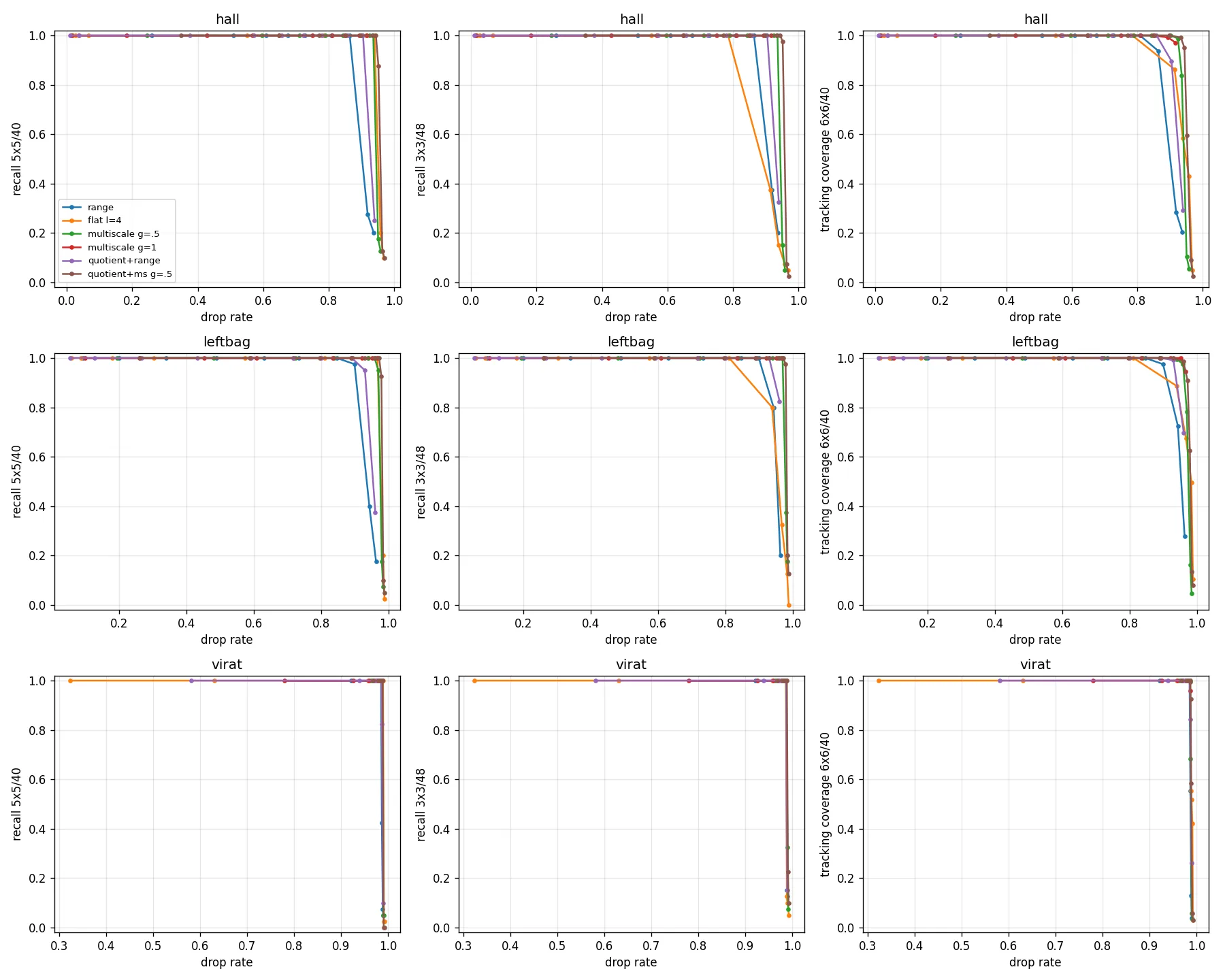
- The multi-scale certificate is the main gain: 2.5 to 3.5 times fewer kept patches at equal recall on the noisy cameras. Noise averages away over a box, a jittering one-pixel edge dilutes by the box width, and a compact object does not. The certificate is weaker in exactly one way: it covers objects that contain a box of the given size at that scale's contrast, not single pixels. The 3×3 objects are still caught at 100 %.
- The quotient certificate adds a consistent 4 to 5 points on top, and is the only one that attacks jitter at its cause.
- Transport does not help. At its high-drop settings the flat norm's recall on 3×3 objects is 0.10 to 0.33.
- The cost. Mover coverage dips to 0.91 to 0.95 for the combined rule: a 6×6 object moving 2 px per frame is partly explained as sub-pixel motion and partly diluted. It is still kept on more than nine frames in ten, and the certificate says so explicitly. A tracker that needs every frame should use quotient + range.
- On a clean camera every rule sits at the 98 to 99 % ceiling. The alternatives matter where the original rule was weakest.
The theorems are checked in the test suite: dual-feasible test functions never exceed the flat-norm bound; box statistics match brute force and the multi-scale bottleneck bound holds on every dropped patch of a test sequence; the quotient rule's and bottleneck certificates hold against the warped view; and the C++ quotient pruner matches numpy bit for bit on keep masks.
9The time axis: a sequential certificate
Every rule so far is memoryless. It compares one frame with the reference and cannot see a change fainter than one frame's noise. Sequential analysis is the branch of statistics built for exactly this: Page's CUSUM [2], Lorden's minimax formulation [3], Moustakides' proof that CUSUM is exactly optimal [4], and Lai's window-limited generalised likelihood ratio for unknown post-change parameters [5]. Its theorems say how early a persistent change can be detected at a given false-alarm rate, and which statistic achieves it. To my knowledge it has not been applied to token skipping.
Setting. Per patch, after the last keep at time , the quotient residuals are observations. "No change" means mean zero, up to the reference's own fixed noise, which is static and cancels below. "Change at " means a persistent mean shift on some region for . The time, place, size and magnitude of the change are all unknown.
9.1The statistic
For window lengths (dyadic) and box half-widths , let be the mean of over the last frames and the mean over the frames before those:
For a Gaussian mean shift at a known time, place and size this is the log-likelihood ratio up to a monotone map. Maximising over is the generalised likelihood ratio, and restricting to dyadic windows is Lai's window limitation. Spatially it is the box scan of Rule 2, and Arias-Castro, Donoho and Huo [6] prove such scans are minimax-optimal for detecting geometric objects in noise.
9.2Self-normalisation: what the footage forced
Measured on three cameras, the per-pixel residual noise looked white but was spatially correlated, along scan lines on the analog camera and in codec blocks on the others, and on the two codec clips its variance grew with the window length. Under such noise the Gaussian scale is wrong by a factor of 2 to 3 at long windows, and the box statistic fired on 40 to 90 % of static patch-frames.
The remedy is classical: self-normalise. Let be the extreme statistic per patch. Its null location and spread are learned per patch from quiet frames, those on which neither rule fires, and the test is
Standardising the maximum and not the field is deliberate. A scale estimated from overlapping box positions is biased low by their correlation (measured: 15 %), whereas the empirical distribution of over time is nonparametric in the noise's spatial correlation and temporal spectrum. A planar illumination term is projected out per patch before accumulation, so that smooth lighting drift is not mistaken for an object.
Proposition 7 (false fires).
If the noise is stationary and the null of is Gumbel-like with location and spread , as for the maximum of many weakly dependent variables, then for each patch, frame and test
and the union bound applies over the tests. At this is about per patch-frame.
Measured: on white noise and on the hallway camera. With independent Gaussian noise and the parametric scale one would have the a-contrario bound with , the "number of false alarms" of Desolneux, Moisan and Morel [7]. That is the bound the footage violated.
Proposition 8 (detection delay).
A persistent object of contrast containing a -box that appears at frame is kept by frame , for the smallest with
with probability at least the null tail at .
Proof.
At the recent window lies entirely after the change and the earlier window entirely before it. The box centred on the object therefore has less the leakage of the planar projection, and is at least that.
On the hallway camera the learned null at has and grey levels. At a persistent object of contrast about 2.5 grey levels is detectable within four frames. The memoryless certificate at the same operating point needs for the same 5×5 box.
Optimality. No procedure can detect reliably while
the minimax lower bound for a box of unknown position and scale in Gaussian noise [6], which in time is Lorden's bound [3]. The delay of Proposition 8 is within a constant factor of the best possible, and the dyadic rounding within a factor 2.
What is certified. The sequential test only adds keeps to the memoryless rule, so every dropped patch still carries the worst-case certificate of Theorems 5 and 6. What it adds is a statistical guarantee no memoryless rule can have: a persistent faint change is kept within a provable, near-optimal delay. Reference noise and static bias cancel in , independent noise averages down by , and what does not cancel is real, persistent change.
9.3Two guards the wider footage forced
On codec-clean cameras static blocks repeat exactly between frames. The learned spread collapses to numerical zero, and the codec's periodic requantisation, every 6 to 12 frames on the VIRAT 720p scenes, fires 94 % of the patches at once. One scene lost eleven points of drop rate to it.
- A physical floor on the spread, with grey levels. A box-mean statistic cannot be resolved below a fraction of a quantisation step, so a narrower null is an artefact of the data and not of the scene.
- A global-coincidence veto. If more than a fraction of all patches fire in the same frame, the event is scene-wide (a keyframe, an illumination change) and not an object. No patch is kept and the frame is used to train the null. Under the independence that Proposition 7 assumes, the expected number of simultaneous false fires is far below that fraction, so the veto does not trigger on noise, or on objects that cover a small part of the frame. A faint change that covers more than a tenth of the frame at once, such as haze or smoke, is vetoed along with the keyframes. That case was not tested.
Measured, the two guards restore the lost drop rate exactly (0.883 → 0.998) and leave faint-object recall unchanged.
9.4Results
New planted events: 45 faint persistent objects per clip, 6×6 px at contrast 8, 12 or 16, present for 3 s. Recall means kept within 1 s of appearance.
An offline oracle bounds what is achievable. The fraction of patch-frames with real change according to a temporal-median background that no online rule can use ( on at least 8 px, 3-frame majority) is 0.081 on the hallway, 0.034 on the lobby and 0.014 on VIRAT. The rules below keep 0.055 to 0.059, 0.027 to 0.029 and 0.012 to 0.015: at or below the oracle, because a person who pauses needs no new token. There is no drop-rate headroom left. The gains from here are in what gets seen.
Table 5. Faint-object recall, with each rule at the threshold giving 100 % recall of the objects of Table 4. The last two rules of each clip sit at nearly the same drop rate; the range rule keeps more patches at that threshold, as the drop column shows.
| rule | clip | drop | faint 8 | faint 12 | faint 16 | mover coverage |
|---|---|---|---|---|---|---|
| range | hallway | 0.808 | 0.27 | 0.33 | 0.47 | 1.00 |
| quotient + multi-scale | hallway | 0.944 | 0.00 | 0.13 | 0.33 | 0.94 |
| + sequential, | hallway | 0.941 | 0.93 | 1.00 | 1.00 | 0.95 |
| range | lobby | 0.847 | 0.53 | 0.67 | 0.67 | 1.00 |
| quotient + multi-scale | lobby | 0.973 | 0.13 | 0.07 | 0.20 | 0.90 |
| + sequential, | lobby | 0.971 | 1.00 | 1.00 | 1.00 | 0.90 |
| range | VIRAT | 0.984 | 0.00 | 0.07 | 0.07 | 1.00 |
| quotient + multi-scale | VIRAT | 0.988 | 0.00 | 0.07 | 0.07 | 0.90 |
| + sequential, | VIRAT | 0.985 | 0.93 | 1.00 | 1.00 | 0.90 |
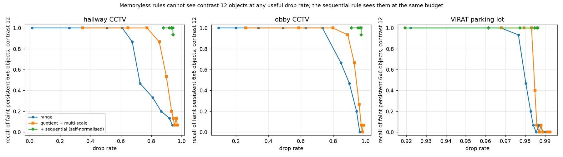
The range rule's non-zero faint recall is luck: contrast 8 to 16 is below its threshold of 40, and it fires when noise happens to add to the object within the one-second horizon. The sequential rule's recall is by design, on the first frame, for 0.2 to 0.4 points of drop rate. Sweeping from 4 to 12 moves the hallway drop rate from 0.88 to 0.943 with faint-12 recall at least 0.93 throughout; is the knee on all three cameras.
After the two guards were added, at the drop rates are 0.943 / 0.972 / 0.987 and faint recall at contrast 8 / 12 / 16 is 0.87 / 0.93 / 1.00 (hallway), 0.93 / 1.00 / 1.00 (lobby) and 1.00 / 1.00 / 1.00 (VIRAT). The guards cost nothing here.
False fires on oracle-static patches: 0.13 % of patch-frames at and 0.03 % at ; on white Gaussian noise 0.03 %. The C++ sequential pruner matches numpy keep for keep: 0 of 118,800 patch decisions differ on the planted hallway clip.
The model matters. The first implementation used the parametric Gaussian scale and failed on all three cameras, with a drop rate of 70 % where 95 % was expected. The self-normalised version is the one reported. Its guarantees are statistical and conditional on stationarity of the camera noise over the learning window; illumination flicker that is neither smooth nor static is treated as change, correctly.
10From patches to pixels: masks in real time
The skip rules decide per 16×16 patch. A segmentation mask is a decision per pixel. The goal was masks of the quality of a semantic-segmentation figure, with filled silhouettes, a flat background, one colour per object and no class labels, produced on video at video rate.
10.1One frame: an exact Potts solution
The natural per-frame formulation is a Potts model: label each pixel foreground or background, balancing the evidence against the length of the boundary. A theorem of Chan, Esedoğlu and Nikolova [8] makes it exactly solvable. The convex relaxation
has, by the coarea formula, a global minimiser whose every superlevel set , , is a global minimiser of the binary problem. Here is the studentised, shadow-suppressed residual evidence, negative where the change is significant, and makes the boundary cheap exactly where the residual has an edge, so silhouettes snap to objects. Chambolle–Pock [9] solves it; sixty iterations per frame give a converged mask.
10.2A video: track the minimiser
Solving each frame from scratch treats a video as a pile of photographs. The energy at frame differs from the energy at by a small drift of the evidence, and its minimiser by a small motion of the objects. Treat it as what it is, a time-varying convex optimisation [10], and track the minimiser:
The proximal term is the video prior, labels move continuously, and it makes -strongly convex. The prediction advects each tracked object by its own velocity, estimated from the displacement of its centroid. The correction is primal–dual steps from that warm start.
Proposition 9 (tracking error).
Let minimise , let be the contraction factor of one primal–dual step on the strongly convex problem, and let be the prediction error. After steps,
a fixed multiple of one frame's unforeseen drift, independent of the length of the video.
Proof.
Contraction of the fixed-point map toward , the triangle inequality through , and a geometric series. This is the prediction–correction bound of [10] specialised to a fixed step count.
Event-driven correction. Which pixels can have moved? Those where the evidence changed coherently (the multi-scale statistic on the residual, at half its certified threshold), those near an object's current or predicted position, those whose labels were not stationary last frame, and a one-patch halo. Only there are the primal and dual variables updated. Elsewhere , the dual variable and the mask are reused. This is the segmentation analogue of the skip rule: work scales with what changed and not with the frame.
Proposition 10 (certificate for reused labels).
is convex, so a point is optimal iff the KKT residual vanishes everywhere. For each pixel,
must be where , where and where , with . The residual is evaluated on the active set every frame, and on each frozen patch when it was last touched; a frozen patch is reactivated as soon as its residual exceeds . Hence at every frame the whole labelling, frozen region included, is -stationary for the current energy, and the gap to the exact minimiser is bounded by the residual times the diameter of .
10.3Three additions for crisper masks
Lagrangian evidence accumulation. Section 9 accumulated evidence per patch to see faint persistent objects. The same idea works per pixel once the accumulator moves with the object. Let be the signed studentised residual and the tracked velocity of the object covering :
Lemma 11.
If has unit variance and is independent across frames, has variance , so again has unit variance under the null. If persists along the object's trajectory, then and
which is for .
Proof.
A geometric series for the mean. For the variance, has fixed point .
The unary term uses : strong instantaneous evidence is kept and persistent weak evidence is doubled. Without the advection, a fast object leaves a trail of accumulated evidence behind it.
Boundary weights from both residual and image. with . A boundary is cheap wherever either the residual or the image has an edge, which is where an object's contour lies.
Guided-filter snap. After clean-up the binary mask is passed through the guided filter of He, Sun and Tang [11] with the frame as guide, in a band around the contour, and re-thresholded at ½. The filter fits a local linear model in each window, so the contour moves onto the nearest intensity edge and leaves textureless regions alone. Being a weighted average of the mask, it cannot create foreground far from the contour, and it is per pixel.
Ghosts. When an object is present during background initialisation, or sits still long enough to be absorbed, the spot it later vacates differs from the model. A ghost and an object are told apart by where their outline lives: a ghost's outline is in the background model and absent from the frame ; a real object's is in and absent from . For each component the contour contrast is measured on both images, and a component whose contrast in is below a floor, or below 0.6 of its contrast in , is a ghost. It is not reported and its pixels are absorbed at rate 0.25 per frame. The second source of ghosts is removed at the root: objects are no longer absorbed into the background while they are objects. A parked car or an abandoned bag therefore remains an object, as it should.
10.4Results
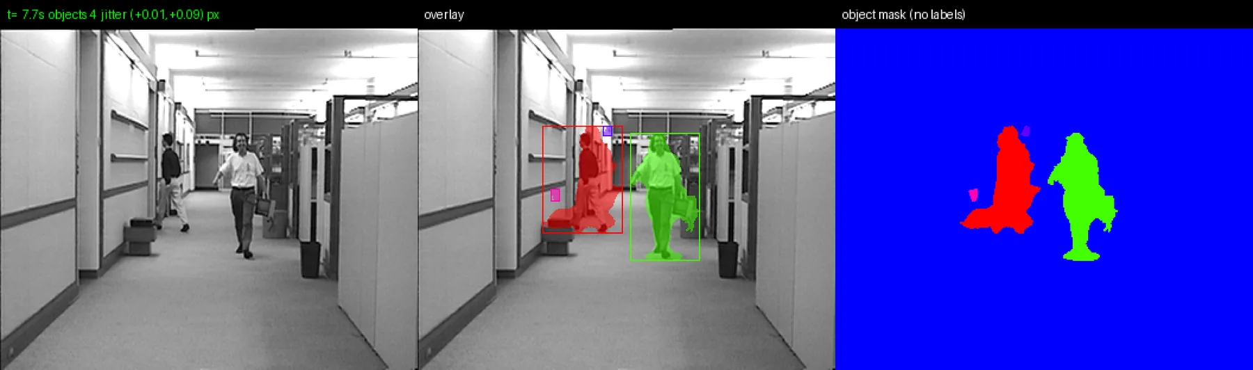

Fidelity of tracking against solving. On the hallway camera, with the same evidence, the tracked mask at 3 steps per frame against the fully converged per-frame solution (150 iterations) has mean IoU 0.938 and median 0.957, with 3 % of frames below 0.8. The KKT residual on the frozen region stays at or below 0.050 on every frame of the final runs, by construction of the reactivation rule. C++ against numpy on the same clip: mean IoU 0.987 to 0.993. Both figures compare the tracker with the method's own solutions. No mask here is scored against human-labelled ground truth.
Table 6. Speed of the tracker, C++, Apple M4, rendering excluded. The cost follows the active set, not the resolution.
| clip | resolution | active set | ms / frame | fps |
|---|---|---|---|---|
| hallway (Xiph) | 352×288 | 49 % | 7.1 | 140 |
| mall corridor (CAVIAR) | 384×288 | 29 % | 6.2 | 161 |
| lobby (CAVIAR) | 384×288 | 23 % | 5.6 | 178 |
| parking lot (VIRAT), full 70 s | 1280×720 | 4.6 % | 34.0 | 29 |
| building forecourt (VIRAT) | 1920×1080 | 5.0 % | 35–42 | 24–29 |
| street with foliage (VIRAT) | 1920×1080 | 9.5 % | 52–55 | 18–19 |
For comparison, the per-frame full solve in numpy at 60 iterations runs at 15.7 fps at 352×288, and the numpy tracker at 38 fps. Sixty iterations are replaced by three, and full frames by the one pixel in twenty the evidence actually touches. At 1080p the per-patch stages run in parallel in a four-colour schedule: patches of one colour are never adjacent, so no two threads write the same pixel. About 24 ms of the 1080p frame time is fixed full-frame work (jitter fit, illumination, background and noise update, component labelling), which is the next thing to make sparse.
Quality, plainly. Silhouettes are filled and stable, shadows on flat floors are suppressed, a car crossing a parking lot is one clean blob. Identity through contact is handled by the tracker and not by connected components: when one component overlaps two substantial predicted objects it is partitioned by nearest predicted object, so two people walking shoulder to shoulder keep separate masks.
What classical evidence cannot do: a grey coat against a grey wall thins the silhouette at the waist; people who enter the scene already touching share one identity until they separate; a polished pillar that reflects passers-by is segmented as change, because it is one; far-away people a few pixels tall are at the mercy of the minimum-area setting; and a person who stands still through background initialisation is background. A learned segmenter would beat this on appearance. Nothing here is learned, and every mask comes with the statement that it is an -stationary point of a convex energy whose data term is a calibrated statistical test.
11A negative result: predictive look scheduling
Where prediction could pay. At the patch level the certified rule already decides before any token is computed, so predicting a skip saves a few arithmetic operations and nothing else. One level up, a video model decides when to look at the stream, and today it does so blind, at a fixed 1 to 2 fps. A scheduler that lengthens its horizon when the scene is quiet and shortens it when things happen would save decoding and lower delay. Nothing deterministic can be certified about frames nobody looked at, so the only honest guarantee is distribution-free and statistical.
Setting. After a look at frame , choose a horizon , skip frames, and look again. Define a miss as iff and the refreshed set contains at least patches outside the one-patch dilation of the set that was active at the previous look: an onset arrived, in a region not being tracked, while we were not looking. Ongoing activity is not a miss; its staleness is reported separately.
Policy. With the running estimate of the onset rate per frame in activity state ,
The predicted onset probability per window is in every state, and the multiplier is an online integrator on the miss rate, one per state. This is the update of Gibbs and Candès [12] in the log-horizon domain. The later critique that it is a control property and not conformal inference is correct, and the name used here is the honest one.
Proposition 12 (one-sided, deterministic, distribution-free).
For any frame sequence, within each state with decisions,
Proof.
The ceiling can only lower , so unless the floor binds. The floor could bind only when at a where the horizon is already 1, and there by definition, so it never binds. Summing and bounding gives the statement.
No lower bound is claimed. In a quiet scene the horizon saturates at and the miss rate stays below , which is the desired behaviour.
Proposition 13 (the structural limit).
If onsets form a memoryless process with rate independent of the observable state, then for any schedule with mean horizon the expected miss rate is to first order, and the mean staleness of motion is
with equality iff the schedule is uniform. Hence no adaptive schedule improves on uniform sampling in (looks, misses, staleness), and adaptivity can pay only through state-dependence of the onset rate.
Proof.
The miss probability is linear in for small . Jensen's inequality gives the staleness bound.
What the footage says. Native frame rate, per-patch rule quotient + multi-scale at , a miss defined as an onset of at least 3 new patches, .
Table 7. Adaptive scheduling against uniform sampling at the same cost.
| clip | onset rate, quiet / active | best uniform at 10 % miss | adaptive : looks/s, miss, staleness | uniform at equal cost: miss, staleness |
|---|---|---|---|---|
| mall corridor | 0.17 / 0.40 | none below | 23.2, 0.040, 0.07 | 0.044, 0.05 |
| lobby | 0.11 / 0.24 | none below | 21.4, 0.046, 0.14 | 0.065, 0.11 |
| VIRAT parking lot | 0.0037 / 0.0076 | (3 looks/s) | 3.6, 0.027, 6.64 | 0.040, 3.82 |
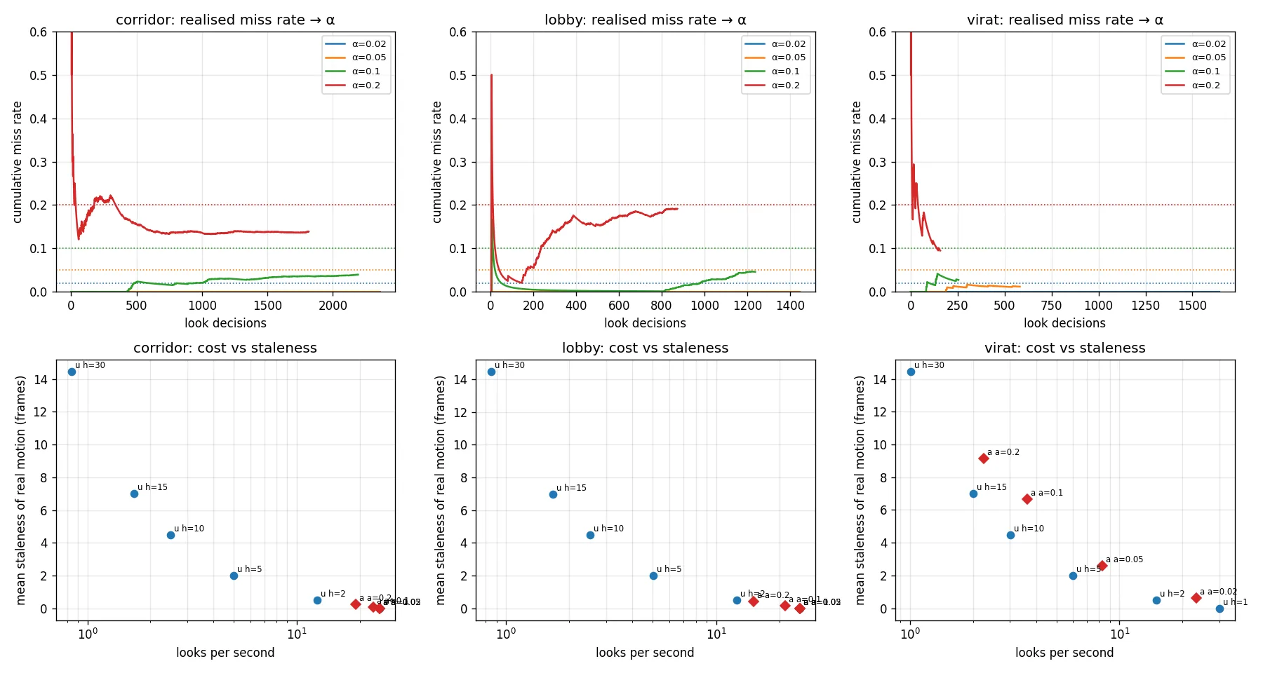
The guarantee held in 12 of 12 runs. An adversarial test in which an opponent plants an onset in every skipped window cannot push the miss rate above the bound, and the scheduler converges to looking at every frame. For memoryless onsets at rate the learned horizon converges to .
Verdict. Sound, self-calibrating, and not better than a tuned uniform rate on real surveillance footage. On busy indoor cameras new activity appears in 17 to 92 % of frames, so no schedule can skip under a 10 % miss constraint. On the quiet parking lot the onset rates in quiet and active states differ only by a factor of 2 to 3, so there is little for the scheduler to exploit: at equal cost it ties uniform on misses and is worse on staleness, exactly as Proposition 13 predicts.
This is the result that justifies the main design. Looking at every frame with the cheap certified statistic costs almost nothing and makes the deterministic certificate possible, which no predictive scheme can offer.
12Breadth: 25 fixed-camera clips
Every fixed-camera clip available was run at the thresholds fixed in advance from Sections 8 and 9: range at , quotient + multi-scale at , sequential at . The floor and the veto of Section 9 were not fixed in advance. The first pass over these clips is what showed they were needed, and the sequential columns below are the rerun with both in place, so they are not a held-out result. Up to 600 frames per clip at native rate, which is 20 to 25 seconds per camera; VIRAT scenes analysed at 960×544. Planted per clip: 20 small, 20 tiny, 10 fades and 10 faint persistent objects (6×6, contrast 12).
Table 8. All 25 clips. Oracle change is the fraction of patch-frames with real change according to an offline temporal-median background. The last column is recall of contrast-12 persistent objects without and with the sequential layer.
| clip | source | res. | fps | oracle change | range | quotient + MS | + sequential | faint-12: MS / seq | |
|---|---|---|---|---|---|---|---|---|---|
| VIRAT 000200_00 | VIRAT | 960×544 | 30 | 0.00 | 0.015 | 0.989 | 0.992 | 0.991 | 0.00 / 1.00 |
| VIRAT 000200_01 | VIRAT | 960×544 | 30 | 0.00 | 0.013 | 0.986 | 0.991 | 0.991 | 0.00 / 0.90 |
| VIRAT 040000_00b | VIRAT | 960×544 | 30 | 0.00 | 0.014 | 0.990 | 0.998 | 0.998 | 0.00 / 1.00 |
| VIRAT 050000_05 | VIRAT | 960×544 | 30 | 0.00 | 0.065 | 0.950 | 0.966 | 0.965 | 0.10 / 1.00 |
| akiyo | Xiph | 352×288 | 30 | 0.00 | 0.182 | 0.927 | 0.972 | 0.971 | 0.20 / 1.00 |
| EnterExitCrossingPaths1 | CAVIAR | 384×288 | 25 | 0.30 | 0.104 | 0.935 | 0.961 | 0.959 | 0.10 / 0.90 |
| Fight_Chase | CAVIAR | 384×288 | 25 | 0.37 | 0.055 | 0.820 | 0.964 | 0.964 | 0.20 / 1.00 |
| LeftBag | CAVIAR | 384×288 | 25 | 0.46 | 0.038 | 0.816 | 0.971 | 0.970 | 0.20 / 0.90 |
| Meet_Crowd | CAVIAR | 384×288 | 25 | 0.40 | 0.029 | 0.821 | 0.973 | 0.972 | 0.00 / 0.90 |
| OneLeaveShopReenter1 | CAVIAR | 384×288 | 25 | 0.37 | 0.059 | 0.956 | 0.974 | 0.971 | 0.10 / 0.90 |
| Walk1 | CAVIAR | 384×288 | 25 | 0.45 | 0.039 | 0.828 | 0.974 | 0.974 | 0.40 / 1.00 |
| WalkByShop1 | CAVIAR | 384×288 | 25 | 0.32 | 0.062 | 0.963 | 0.981 | 0.980 | 0.30 / 1.00 |
| hall_monitor | Xiph | 352×288 | 30 | 1.69 | 0.081 | 0.784 | 0.949 | 0.948 | 0.10 / 1.00 |
| VIRAT 010000_02 | VIRAT | 960×544 | 24 | 0.00 | 0.024 | 0.980 | 0.995 | 0.995 | 0.10 / 0.90 |
| VIRAT 010106_01 | VIRAT | 960×544 | 24 | 0.00 | 0.018 | 0.990 | 0.997 | 0.996 | 0.00 / 0.90 |
| VIRAT 010109_00 | VIRAT | 960×544 | 24 | 0.00 | 0.061 | 0.971 | 0.996 | 0.996 | 0.10 / 1.00 |
| VIRAT 010112_00 | VIRAT | 960×544 | 24 | 0.00 | 0.067 | 0.983 | 0.996 | 0.996 | 0.10 / 1.00 |
| VIRAT 010200_02 | VIRAT | 960×544 | 24 | 0.00 | 0.006 | 0.996 | 0.999 | 0.999 | 0.00 / 1.00 |
| VIRAT 010204_01 | VIRAT | 960×544 | 24 | 0.00 | 0.017 | 0.988 | 0.993 | 0.993 | 0.10 / 1.00 |
| VIRAT 040000_02 | VIRAT | 960×544 | 30 | 0.00 | 0.010 | 0.992 | 0.999 | 0.999 | 0.10 / 1.00 |
| VIRAT 040103_08 | VIRAT | 960×544 | 30 | 0.00 | 0.013 | 0.985 | 0.995 | 0.994 | 0.00 / 1.00 |
| VIRAT 050201_03 | VIRAT | 960×544 | 30 | 0.00 | 0.232 | 0.953 | 0.990 | 0.989 | 0.30 / 1.00 |
| VIRAT 050300_00 | VIRAT | 960×544 | 30 | 0.00 | 0.286 | 0.887 | 0.974 | 0.973 | 0.30 / 0.90 |
| bridge_close | Xiph | 352×288 | 30 | 1.07 | 0.113 | 0.756 | 0.908 | 0.908 | 0.40 / 1.00 |
| bridge_far | Xiph | 352×288 | 30 | 1.25 | 0.000 | 0.886 | 0.997 | 0.997 | 0.00 / 0.90 |
Table 9. Summary over the 25 clips.
| range, | quotient + multi-scale | + sequential | |
|---|---|---|---|
| median drop rate | 0.956 | 0.990 | 0.989 |
| minimum drop rate | 0.756 | 0.908 | 0.908 |
| recall, small / tiny / fading | 1.00 / 1.00 / 1.00 | ||
| recall, faint contrast 12 | 0.13 | 0.96 |
The cost of the sequential layer over quotient + multi-scale is at most 0.003 and 0.001 at the median. It was eleven points on one scene before the two guards of Section 9.
At and the worst-case certificate behind the last two columns is contrast 80 for a single pixel, 46 for an object that contains a 3×3 box, 36 for 5×5 and 30 for 7×7. That is a weaker statement than Theorem 1 at , which is the first column.
On the 15 codec-clean clips, where static blocks repeat exactly and , the full rule drops between 96.5 % and 99.9 %, and 99 % or more on 11 of them. Fourteen of the 15 are VIRAT scenes, where the MPEG-4 encoder had already frozen the static blocks, so much of the redundancy was removed before the rule saw the frame. The lowest numbers are honest ones: a river camera whose water moves (oracle change 11 %, drop 90.8 %), two busy scenes with 23 to 29 % of patch-frames in real motion, and the analog hallway.
Not covered: night and bad weather. The ChangeDetection 2014 server was unreachable when the breadth run was made, so those clips are the next to add. The heavy-tailed analog cameras here (hallway, bridges) are the closest proxy for what they will do to the range rule.
13End to end with a video language model
Model. Qwen2-VL-2B-Instruct [15], unmodified, on Apple's MPS backend, 2.3 s per query.
Protocol. The model is shown the view a pruning rule leaves it: kept patches at truth, dropped patches at their last kept content. For the two certified rules that is the view of Rules 1 and 3, the last kept content moved by the fitted sub-pixel shift with the brightness shift added. The consecutive-frame rule has no such terms, and its view is the last kept content alone. This isolates the information content of the pruning decisions from the mechanics of token reuse and needs no change to the model. The model processes a full image every time, so nothing is saved in this experiment; the savings a deployment could reach are the drop rates of the earlier sections. Three rules run at the same drop rate per clip: a consecutive-frame mean rule of the EVS and run-length kind, calibrated to the certified rule's drop rate; the certified quotient + multi-scale rule; and the certified rule with the sequential layer.
13.1Does certified pruning change the model's answers on ordinary footage?
Fifteen frames per clip, "How many people are visible?" and "Is there a person visible?", scored as agreement with the model's own answer on the full frame.
Table 10. Agreement of the people count with the full-frame answer, and mean absolute deviation (MAD) of the count.
| clip | drop rate, all rules | consecutive-mean view | certified view | + sequential |
|---|---|---|---|---|
| hallway | 0.949 | 1.00 / 0.00 | 1.00 / 0.00 | 1.00 / 0.00 |
| lobby | 0.979 | 0.47 / 0.53 | 0.93 / 0.07 | 0.87 / 0.13 |
| VIRAT parking lot | 0.996 | 0.80 / 0.27 | 0.80 / 0.27 | 0.80 / 0.27 |
Person-presence agreement was 0.93 to 1.00 for every rule. On the lobby the heuristic view changes the model's people count on half the frames at a 97.9 % drop rate. The certified view, whose every dropped patch is within the contrast certificate of the truth, changes it on one frame in fifteen. On VIRAT the three views agree with each other on every frame, and the 0.80 is the model's own instability on far-away people.
13.2The fade-in blind spot, end to end
A square of contrast 70 fades in over 6 to 8 s, at 0.4 to 0.9 grey levels per frame, far below any consecutive-frame threshold. The square contrasts against its local surroundings and is 48 px wide at CIF and 96 px on the parking lot. Sixteen trials per clip, 48 in all.
Table 11. The fade-in experiment. The model-level rows are conditioned on the model perceiving the object in the truth frame, which it does in 26 of 48 trials.
| hallway | lobby | parking lot | all 48 trials | |
|---|---|---|---|---|
| object present in view at end of fade: consecutive-mean / certified / sequential | 0.12 / 1.00 / 1.00 | 0.25 / 1.00 / 1.00 | 0.00 / 1.00 / 1.00 | 6 / 48 / 48 |
| trials in which the model perceives the object in the truth frame | 8 | 12 | 6 | 26 |
| of those, model answers yes on the consecutive-mean view | 0.12 | 0.08 | 0.00 | 2 / 26 |
| of those, model answers yes on the certified view | 0.75 | 0.92 | 1.00 | 23 / 26 |
| of those, model answers yes on the sequential view | 1.00 | 0.92 | 0.83 | 24 / 26 |
| false "yes" on the no-object control | 0.00 | 0.00 | 0.00 | 0 / 48 |
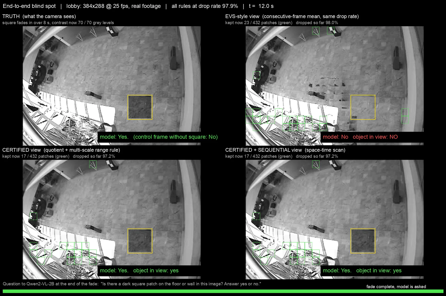
The mechanism is at the pixel level. The heuristic never refreshes a patch that changes by less than its threshold per frame, however large the change becomes. The certified rule refreshes when the accumulated change reaches . The square is larger than a patch. The patches on its border are refreshed. A patch that lies wholly inside it changes uniformly, which is no reason to refresh under any rule here, and it shows the square in the view through the shift .
Verdict. With every rule at the same drop rate, an object that fades in slowly reaches the model's answer through the certified rule in 23 of 26 perceivable cases and through the consecutive-frame rule in 2 of 26. On ordinary footage the certified view leaves the model's answers as stable as the full frame, or far more stable than the heuristic view.
Limits to state. A 2-billion-parameter model on a laptop. Three cameras. Synthetic squares and not real objects: the model perceives them in only 26 of 48 truth frames, which is why the metric is conditioned. Views and not actual token reuse inside the model, and the certified views use the shift , which a cached token does not carry.
The only baseline is the consecutive-frame rule. Mean against last kept, which caught every fade in Table 2, was not run here or in Sections 8, 9 and 12. A consecutive-frame rule with a full refresh every few seconds would also bound how long a fade can stay unseen, and was not run either. So the pixel-level result, the object present in the view in 48 of 48 trials against 6 of 48, measures the cost of comparing consecutive frames. It does not show that a proof is needed to avoid that cost.
14Implementation and speed
The reference implementation is a header-only C++17 core with a C ABI and a command-line tool that reads raw grey frames on standard input, plus a numpy reference whose keep decisions must match the C++ exactly for the range, quotient and sequential rules, and a Python layer for baselines, the topology checker, noise analysis and the experiments.
The mask tracker agrees with its numpy version to a mean IoU of 0.987 to 0.993, not exactly, and the transport certificate and the look scheduler exist only in numpy.
The code, the tests, the recorded outputs of every run and short demo clips are at github.com/nsquaredzz/certified-skip, under the MIT licence.
Table 12. Throughput on an Apple M4.
| component | implementation | 352×288 | 1280×720 | note |
|---|---|---|---|---|
| range rule | C++ | 836 fps at 1280×534 | full film, decoding included; about 1,150 fps on 1080p synthetic | |
| quotient rule | numpy | 104 fps | ||
| quotient rule | C++, single thread | 1,040 fps | 106 fps | |
| sequential rule | numpy | 59 fps | ||
| sequential rule | C++, single thread | 467 fps | 89 fps | holds frames of prefix sums |
| mask tracker | C++ | 140 fps | 29 fps | 18 to 29 fps at 1920×1080 |
The multi-scale rule is integral images and costs about the same as the range rule. The test suite covers the semantics, native parity, the stability bound, tightness, the audit, calibration, each alternative certificate, the sampler's guarantee under an adversary, and the segmenter.
15What is new, what is not, and what is missing
Not new. Motion-compensated prediction with a residual test is every video codec since H.261. Conditional replenishment is from 1969 [14]. Box filtering and scale-space blob detection are classical. The flat norm is Whitney's. Sequential analysis is from 1954 to 1998. Background subtraction, Potts models, graph cuts, TV relaxations, Chambolle–Pock, morphology and overlap tracking are all standard, and prediction–correction tracking of a time-varying convex program is standard in control and signal processing.
New, to my knowledge.
- The certificate: for each statistic, a theorem naming exactly what cannot have happened in a dropped patch, and a tightness construction showing the threshold cannot be moved.
- The observation that the right thing to quotient out is a motion group, so that stability only has to pay for what the group cannot explain. This is also the route to moving cameras.
- A skip rule that certifies in both directions: worst case, nothing of contrast appeared in a dropped patch; statistically, any persistent change above a few grey levels is kept within a provable, near-optimal delay, with the null measured and not assumed.
- Prediction–correction tracking used to make a segmentation energy follow a video, with the active set driven by the certified change statistic and a KKT certificate for the labels that are reused.
Missing.
- Moving cameras. The quotient certificate generalises to homographies in principle; none of it is implemented or measured.
- Night, rain, snow and thermal footage.
- Real token reuse inside a model. Section 13 measures the information in the view, not latency or memory in a deployed model, and it leaves open how a cached token would receive the brightness shift .
- A larger model and real, not synthetic, slow-appearing objects in the end-to-end test.
- Recall on real, annotated events. CAVIAR and VIRAT are distributed with hand-labelled tracks, and they are not used here: every recall figure is on planted synthetic objects.
- Mean against last kept, and a consecutive-frame rule with a periodic full refresh, as baselines on real footage and in the end-to-end test.
- Long recordings. Each clip is 20 to 25 seconds. Nothing here runs for hours or through a change of lighting.
- Colour. Every rule runs on luma.
- An exact flat-norm solver for audits, and in the topology checker.
16How the project actually went
The order of the sections is the order of the work, and several of the results exist only because something failed first.
- The range rule worked on paper and on clean cameras, and lost a quarter of its drop rate on a noisy one. The Gaussian noise model said this could not happen. An overlay of the kept patches showed strips along wall edges. That one picture set the direction of everything after it.
- Transport looked like the natural fix and was not. A jittering edge is single-signed mass. It was worth the theorem and stays as a baseline.
- The first sequential rule used the textbook Gaussian scale and fired on 40 to 90 % of static patches. Real camera noise is correlated in space and drifts in time. Self-normalising the maximum fixed it.
- The breadth run then broke the sequential rule again, on the cleanest cameras: static blocks repeated exactly, the learned spread collapsed to zero, and codec requantisation fired almost every patch at once. A floor and a veto restored it.
- High-resolution footage broke the mask tracker in three small ways: a per-frame displacement bound of 8 px inherited from CIF silently disabled prediction for cars at 1080p and left a trailing smear (now 48 px); an active-set test on raw grey levels made half the frame active under wind (now studentised, 5 to 10 %); and ghosts appeared where a car had been parked during initialisation. A fourth was a plain bug: an unsized buffer in the C++ ghost code crashed the process on first use. Silent crashes in native code are the first thing to look for when a render script prints nothing.
- The first scheduling benchmark defined a miss as "three or more refreshed patches" and collapsed to looking at every frame, because continuous activity made every window a miss. With the onset definition the experiment became meaningful, and its answer was no.
- The first end-to-end protocol placed bright squares on bright surfaces half the time, and the small model could not see them even in the truth frame. In that run the certified view contained the square in 34 of 36 trials; the two misses were bright squares on the lobby camera. The second protocol contrasts the square with its surroundings, and the metric is conditioned on the model perceiving the object at all.
References
- D. Cohen-Steiner, H. Edelsbrunner, J. Harer. Stability of persistence diagrams. Discrete & Computational Geometry 37, 2007.
- E. S. Page. Continuous inspection schemes. Biometrika 41, 1954.
- G. Lorden. Procedures for reacting to a change in distribution. Annals of Mathematical Statistics 42, 1971.
- G. V. Moustakides. Optimal stopping times for detecting changes in distributions. Annals of Statistics 14, 1986.
- T. L. Lai. Information bounds and quick detection of parameter changes in stochastic systems. IEEE Transactions on Information Theory 44, 1998.
- E. Arias-Castro, D. L. Donoho, X. Huo. Near-optimal detection of geometric objects by fast multiscale methods. IEEE Transactions on Information Theory 51, 2005.
- A. Desolneux, L. Moisan, J.-M. Morel. From Gestalt Theory to Image Analysis: A Probabilistic Approach. Springer, 2008.
- T. F. Chan, S. Esedoğlu, M. Nikolova. Algorithms for finding global minimizers of image segmentation and denoising models. SIAM Journal on Applied Mathematics 66, 2006.
- A. Chambolle, T. Pock. A first-order primal-dual algorithm for convex problems with applications to imaging. Journal of Mathematical Imaging and Vision 40, 2011.
- A. Simonetto, E. Dall'Anese, S. Paternain, G. Leus, G. B. Giannakis. Time-varying convex optimization: time-structured algorithms and applications. Proceedings of the IEEE 108, 2020.
- K. He, J. Sun, X. Tang. Guided image filtering. ECCV, 2010.
- I. Gibbs, E. Candès. Adaptive conformal inference under distribution shift. NeurIPS, 2021.
- P. Indyk, N. Thaper. Fast image retrieval via embeddings. Workshop on Statistical and Computational Theories of Vision, 2003.
- F. W. Mounts. A video encoding system with conditional picture-element replenishment. Bell System Technical Journal 48, 1969.
- P. Wang et al. Qwen2-VL: enhancing vision-language model's perception of the world at any resolution. 2024.
- R. Choudhury et al. Don't look twice: faster video transformers with run-length tokenization. NeurIPS, 2024.
Footage. Xiph.org derf test collection (hall_monitor, akiyo, bridge_close, bridge_far). VIRAT Video Dataset, public release, Kitware. CAVIAR test case scenarios, EC project IST 2001 37540, INRIA and the University of Edinburgh. Tears of Steel, © Blender Foundation, CC-BY.