research · multiverse #002 · 2026-04-28 · revised 2026-10-08 · 21 min read
Escaping Flatland
A hyperbolic context manifold, the mathematics behind it, and what held up when I built and tested it.
Abstract
AI memory and retrieval systems mostly store knowledge in flat vector spaces, even when the knowledge is a hierarchy. This issue proposes a different container. Every coordinate of a node is a point in a Poincare disk, with a magnitude and a phase. Neighbours are combined with a hyperbolic midpoint. Training uses a contrastive loss on hyperbolic distance.
None of the ingredients is new, and the issue says where each one comes from. What it adds is one consistent construction, and a test of it with public code.
Three experiments. First, at low dimension the curved spaces hold far more of a hierarchy: with 8 real dimensions, retrieval precision on the WordNet mammal tree is 0.99 against 0.38 for Euclidean space, which catches up only at 32. Phase alone identifies a concept's branch 99 % of the time; magnitude does not encode depth. Second, the geometry does not stop over-smoothing. Plain layers collapse by 32 layers in every geometry, a skip connection fixes all of them, and the extra depth the proposed layer seemed to give came from its activation and not its curvature. Third, end to end on a tree, link prediction reaches 0.94 to 0.99 AUC for the hyperbolic pipelines at every depth, against 0.97 for the flat one with a single layer and 0.74 to 0.79 with more.
Curved space bought capacity. It did not buy depth.
What changed in this version
The first version of this issue, from April 2026, stated results that had not been measured, and its mathematics had four errors. This version corrects the mathematics, credits the work the idea is built from, and replaces every claim with an experiment that can be rerun. Corrections are marked where they occur. The proposal is the same. The claims are smaller, and one of them turned out to be wrong.
1Hook
A modern AI system can summarize ten papers in seconds and still fail to remember why one paragraph mattered to your project three hours later. It can retrieve "related" chunks yet mix unrelated ideas into one smooth, confident answer. This is not only a model quality issue. Part of it is a geometry issue. We are forcing hierarchical knowledge into a flat space and then acting surprised when structure disappears.
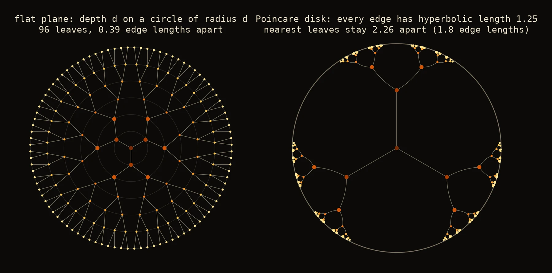
If your memory stack lives in Euclidean embeddings only, deep retrieval starts to behave like semantic averaging. Distances lose meaning as branching depth increases, neighborhoods blur, and graph propagation pushes nodes toward the same latent center. That is the worry this issue starts from. The rest of it is an attempt to make the worry precise, propose a geometry that might help, and then check.
2Where the state of the art is
Today's best production stacks are no longer "vector search + prompt template." They are layered systems: dense retrieval, lexical signals, reranking, graph side channels, metadata filters, and often an agent loop on top. GraphRAG variants, multihop retrievers, and memory-augmented agents have clearly improved recall and answer grounding versus first-generation RAG.
On the representation side, the frontier includes contrastive pretraining, learned retrievers, instruction-tuned embeddings, and graph neural operators. On the reasoning side, tool augmentation and planning loops have improved decomposition of complex tasks. None of that is trivial progress. It is real, hard-earned engineering.
But the dominant geometry is still Euclidean. Even when graph methods are used, aggregation usually happens in a linear latent space. A system can retrieve the right documents and still flatten the concept topology when it fuses them: answers are "close enough" until the task needs precise hierarchy, and then siblings, ancestors and neighbors merge into one blurred explanation.
3Three ways flat memory can fail
I think flat representations fail in three ways. The first two are tested later in this issue. The third is not.
The first is relation collapse. In high-branching domains, Euclidean neighborhoods become overloaded. Concepts that should be separated by depth or role become crowded. Retrieval then surfaces chunks that are semantically adjacent but structurally wrong. Experiment 1 measures this as a capacity question: how much of a hierarchy survives in dimensions.
The second is over-smoothing in graph propagation. Repeated message passing shrinks the differences between nodes until deep stacks lose node identity [17, 18]. This is fatal for a memory system that has to keep provenance paths apart. Experiment 2 asks whether changing the geometry helps.
The third is missing directional relation. Most embeddings encode strength well and relation type weakly. They can tell you two concepts are close, but not how. I come back to this under limits.
4What already exists
Almost every ingredient below has been published, and the first version of this issue did not say so.
- Hyperbolic embeddings of hierarchies. Nickel and Kiela embedded WordNet in the Poincare ball and showed large gains over Euclidean space at low dimension [1]. Sarkar proved that trees embed in the hyperbolic plane with arbitrarily low distortion [2], and Sala et al. turned that into a construction and studied the precision it needs [3].
- Hyperbolic networks. Ganea et al. defined Mobius versions of linear maps, bias and activation [4]. Chami et al. and Liu et al. built graph neural networks on them [5, 6].
- Products of spaces. Gu et al. embed data in products of hyperbolic, spherical and flat factors [7]. The manifold used here is the special case of a product of hyperbolic planes.
- Order-free hyperbolic averaging. The Einstein midpoint comes from Ungar's gyrovector calculus [8]. Gulcehre et al. used it for attention [9] and Shimizu et al. gave its Poincare form [10].
- Complex coordinates and phase. RotatE models a relation as a rotation of phase [12], Chami et al. moved relation-as-rotation into hyperbolic space [13], and MagNet uses a complex Hermitian Laplacian whose phase encodes edge direction [14]. Xiao et al. embed hierarchies in complex hyperbolic space, which is a different manifold from the one here [11].
- Contrastive losses on hyperbolic distance. The loss of Nickel and Kiela is already a softmax over negatives on distance [1], and hyperbolic versions of contrastive learning exist [16].
- Over-smoothing in hyperbolic networks. It has been reported, and treated with residual connections [20].
What this issue adds is small: one consistent way to put these pieces together around complex coordinates, a statement of what each piece is supposed to do, and a test of whether it does.
5The complex lift: Samanya and Samavaya in
The construction begins by separating two quantities that flat embeddings usually entangle. I borrow their names from the Vaisheshika categories: conceptual generality (Samanya) and relational inherence (Samavaya). Instead of storing both in one real coordinate, node features are lifted from into complex coordinates, each with a magnitude and a phase.
Equation 1. The complex lift.
Every coordinate lies inside the unit disk. This is the exponential map at the centre of each disk, applied to .
Correction
The first version wrote the lift as . That lands in the square , whose corners lie outside the unit disk. With unit-variance pre-activations, 31 % of coordinates come out with , where the distance in Equation 2 is undefined.
The design intent is that magnitude says how general a concept is and phase says how it is related to others. Whether a trained model honours that split is an empirical question. Experiment 1 measures it.
6The Poincare bound: hyperbolic geometry
Each coordinate lives in the Poincare unit disk , and a node is a point of the product .
Equation 2. Distance in one disk, and in the product.
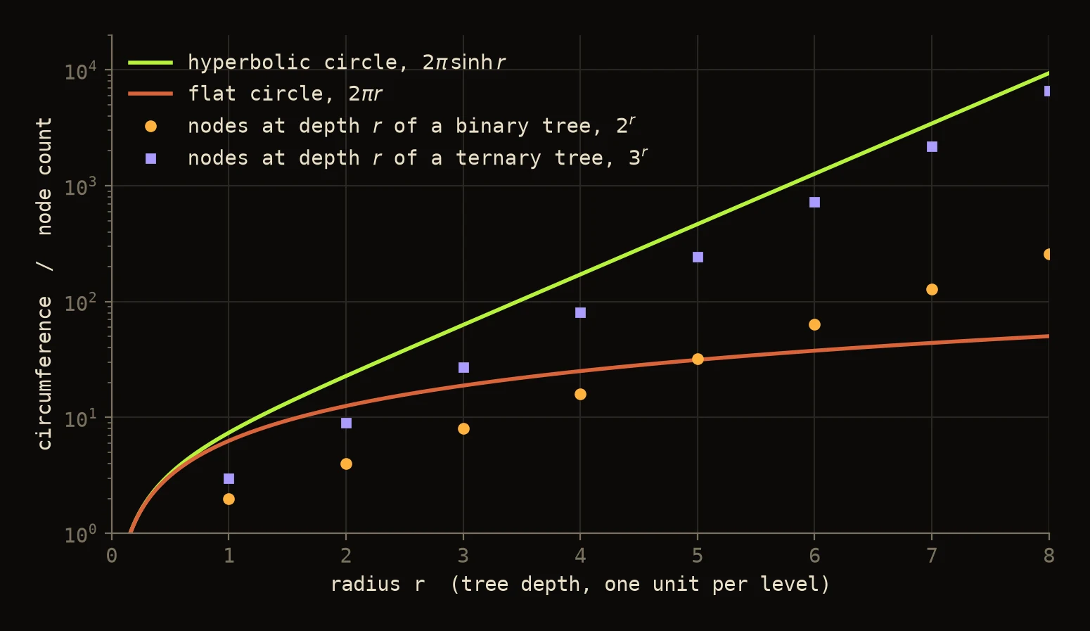
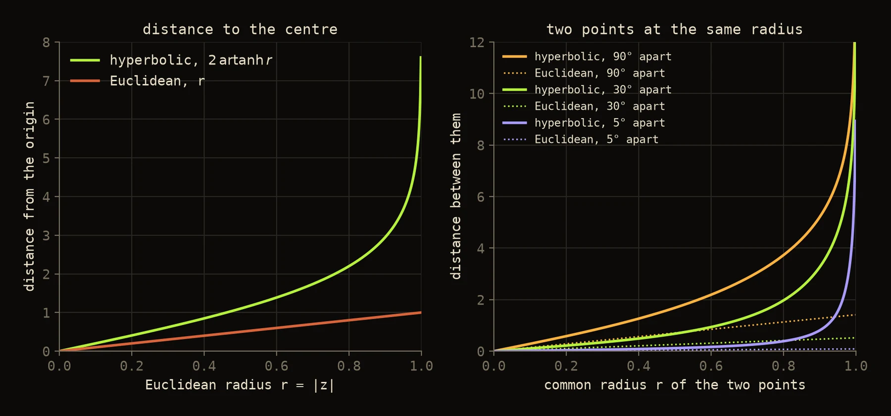
Hyperbolic distance grows rapidly near the boundary. That is what hierarchical memory needs: room for fine-grained leaves near the rim without collisions, and low-radius positions for global abstractions.
Correction
The first version had features in but wrote every formula for a single disk. The product is the reading under which those formulas are correct, one coordinate at a time. It has a cost that should be stated: a product of hyperbolic planes is not itself hyperbolic in the strict sense, because it contains flat planes. The standard alternative is one Poincare ball of the same real dimension [1], so every experiment below includes that ball as a baseline.
7Aggregation without ambiguity
To pass messages, a node has to combine the states of its neighbours. Ordinary addition leaves the disk, so the first version reached for Mobius addition.
Equation 3. Mobius addition in one disk.
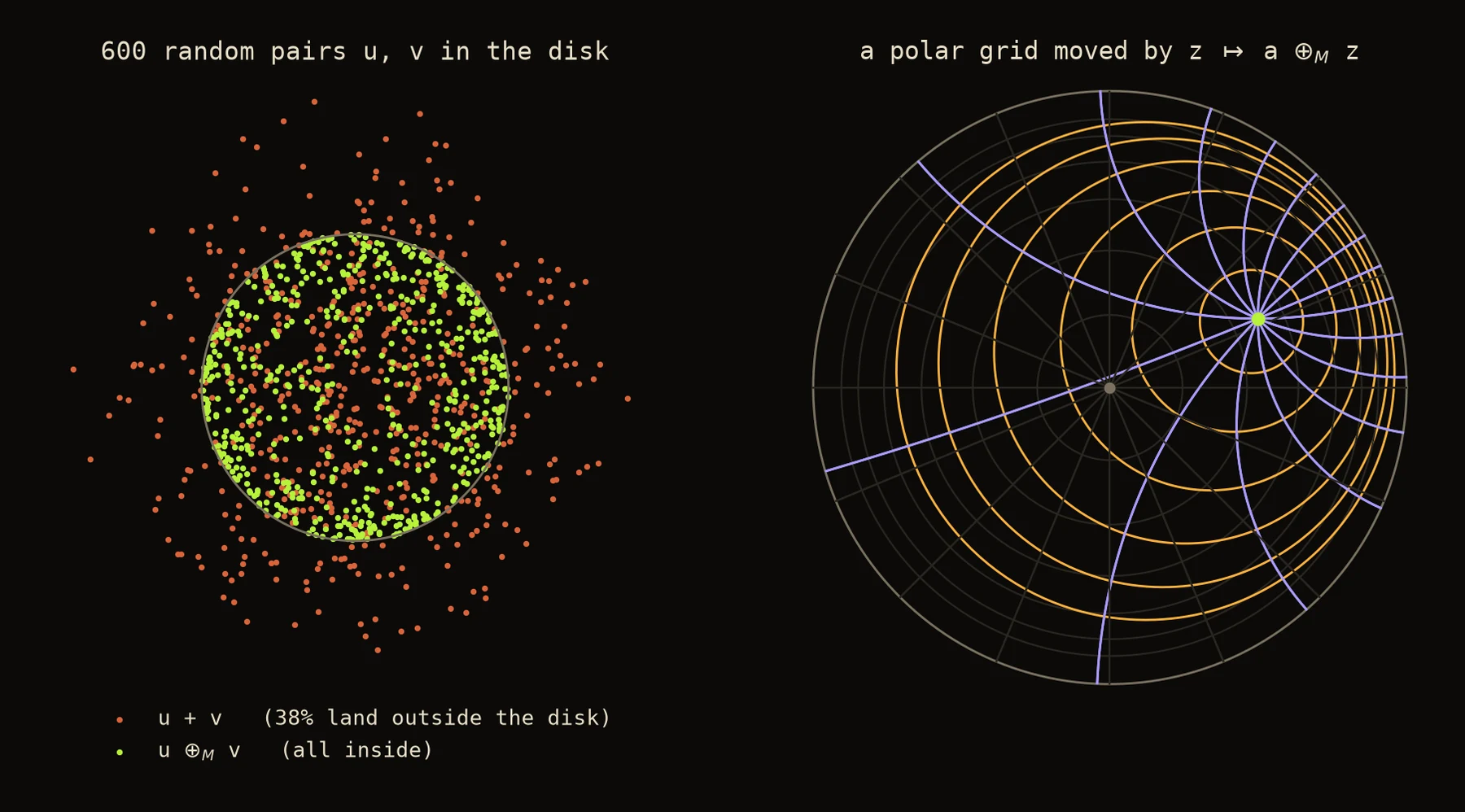
Mobius addition keeps points in the disk and preserves angles. It is also neither commutative nor associative [8]. Swapping the two arguments multiplies the result by , a complex number of modulus one: the order of a Mobius sum shows up as a rotation of phase. That is a problem for a neighbourhood, which has no order. In a test, folding over the same five points in different orders gave results up to 2.2 hyperbolic units apart.
Correction
The first version defined the layer as a Mobius sum over neighbours, , which is not well defined, and called it "Einstein gyrovector addition via Mobius transformations", which names two different operations. The order-free operation is the Einstein midpoint.
Equation 4. The gyromidpoint, and the layer built on it.
This is the Einstein midpoint written in Poincare coordinates, applied in each disk [8, 9, 10]. It does not depend on the order of the neighbours. For two points with equal weights it is the midpoint of the geodesic between them. It commutes with every rotation and every hyperbolic translation of the disk. Each of these is a test in the code. The maps and take a point to the tangent plane at the centre and back, , and is the Mobius matrix-vector product of Ganea et al. [4] with complex weights. The activation gates the magnitude and leaves the phase alone [22].
Phase enters in two places. A complex weight rotates the phase of a coordinate by . And the midpoint adds its arguments as vectors, so neighbours with aligned phases reinforce each other and neighbours with opposed phases cancel.
Correction
The first version said this layer defeats over-smoothing because "the manifold geometry structurally forbids representational collapse into a single degenerate state." That is false. The map that sends every node to one point is as available on the disk as in the plane. And the gyromidpoint is an average: one round over a fully connected neighbourhood puts every node at the same point. Whether a deep stack of these layers stays useful has to be measured. That is Experiment 2.
8The contrastive objective
Reconstruction losses under-constrain topology, so the model is trained to pull related nodes together and push sampled unrelated nodes apart, with similarity given by hyperbolic distance.
Equation 5. Contrastive loss on distance.
With and related pairs as positives this is the loss of Nickel and Kiela [1]. With two augmented views of each node as positives it is the NT-Xent loss of SimCLR [15] with cosine similarity replaced by negative distance. Nothing about it is specific to this manifold, which makes it a fair way to compare spaces: same loss, different .
9Experiment 1: how much hierarchy fits in dimensions?
This is the capacity question behind "relation collapse", and it follows the protocol of Nickel and Kiela [1]. The data is the mammal subtree of WordNet [23]: 1,170 synsets and the 6,448 pairs in which one is an ancestor of the other. Every synset gets a point; there are no features, so the lift of Equation 1 is applied to a free vector per node. Training uses Equation 5 with , related pairs as positives and 10 sampled negatives. Then, for each synset, all others are ranked by distance, and the score is how highly its true relatives rank: mean average precision (MAP), and the mean rank of a true relative among the non-relatives, where 1 is perfect.
Four spaces are compared at the same number of real dimensions , which is the same number of parameters: Euclidean space with distance and with squared distance, the Poincare ball, and the product of disks. The learning rate is chosen per space and dimension from five values on one seed, by the MAP itself, since reconstruction has no held-out set. Each setting is then run with five seeds.
Table 1. Reconstruction MAP on the WordNet mammal hierarchy, mean and standard deviation over 5 seeds. Higher is better.
| real dimensions | Euclidean | Euclidean, squared distance | Poincare ball | product of disks |
|---|---|---|---|---|
| 2 | 0.269 ± 0.001 | 0.132 ± 0.004 | 0.403 ± 0.006 | 0.400 ± 0.005 |
| 4 | 0.306 ± 0.002 | 0.209 ± 0.004 | 0.926 ± 0.003 | 0.836 ± 0.012 |
| 8 | 0.380 ± 0.001 | 0.331 ± 0.002 | 0.958 ± 0.003 | 0.990 ± 0.001 |
| 16 | 0.838 ± 0.001 | 0.864 ± 0.003 | 0.967 ± 0.002 | 0.999 ± 0.000 |
| 32 | 1.000 ± 0.000 | 1.000 ± 0.000 | 0.970 ± 0.002 | 1.000 ± 0.000 |
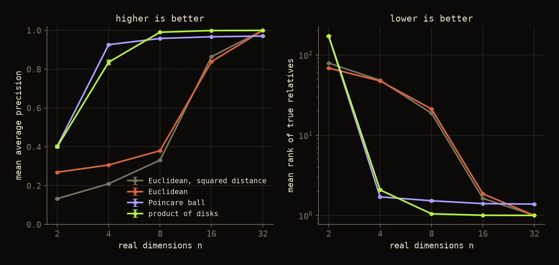
- At low dimension curved space wins by a wide margin. With 8 real dimensions the disks reach a MAP of 0.990 and the ball 0.958, against 0.380 for Euclidean space. In mean rank that is 1.05 and 1.52 against 21.
- Flat space catches up. It reaches 0.84 to 0.86 at 16 dimensions and 1.000 at 32. On a hierarchy of this size the advantage is about the dimension budget, not about what can be represented at all.
- Disks against ball is mixed. The ball is better at 4 dimensions (0.926 against 0.836) and the disks are better from 8 up. I would not read the second half as the product beating the ball: at 16 and 32 dimensions the ball preferred the smallest learning rate tried and was still improving slowly when training ended, so its 0.97 is likely an optimisation limit and not a capacity limit.
- Two dimensions did not work for anyone. One disk scores 0.40 against 0.27 for the plane, with a worse mean rank (171 against 69). With four times the training the disk reaches 0.427 ± 0.011 and a mean rank of 13, against 0.275 and 68 for the plane, and is still rising. The capacity is there in principle [2], and Sala et al. report 0.989 on WordNet in two dimensions from a combinatorial construction [3]. Gradient descent did not find it in this budget.
Three quarters of the synsets are leaves (879 of 1,170), so these scores are mostly a statement about fine-grained leaves.
9.1What magnitude and phase ended up carrying
Equation 1 intends magnitude for generality and phase for relation. The trained disk embeddings let that be checked. Each disk is first re-centred at the root, which removes the freedom to translate the whole embedding. Then two things are predicted by nearest neighbour, once from the phases alone and once from the magnitudes alone: which branch a synset belongs to (the ten subtrees two levels below the root with at least 20 members, such as carnivores, ungulates, rodents and primates), and how deep it sits.
Table 2. Nearest-neighbour accuracy from one channel alone, 1,120 synsets, 5 seeds. Always guessing the largest class scores 0.327 for branch and 0.235 for depth.
| disks | branch, from phases | branch, from magnitudes | depth, from phases | depth, from magnitudes |
|---|---|---|---|---|
| 2 | 0.989 ± 0.004 | 0.421 ± 0.033 | 0.287 ± 0.009 | 0.229 ± 0.019 |
| 4 | 0.995 ± 0.003 | 0.568 ± 0.020 | 0.233 ± 0.008 | 0.261 ± 0.024 |
| 8 | 0.999 ± 0.001 | 0.652 ± 0.016 | 0.148 ± 0.009 | 0.248 ± 0.011 |
| 16 | 0.999 ± 0.001 | 0.697 ± 0.014 | 0.111 ± 0.012 | 0.259 ± 0.010 |
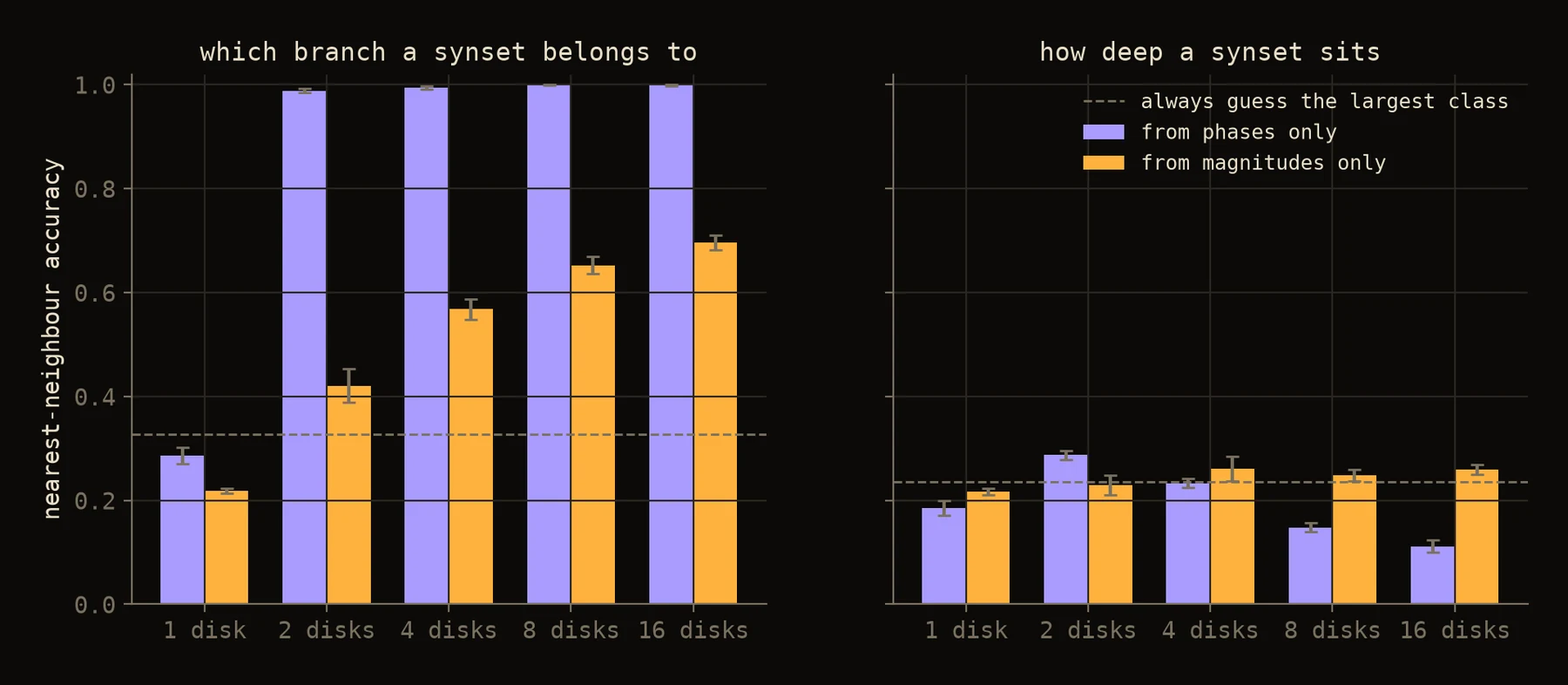
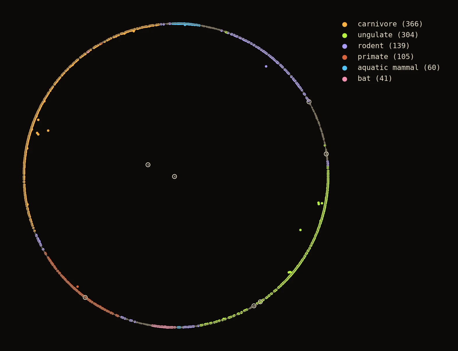
Phase carries branch, as designed. Magnitude does something narrower than designed:
- The root, the most general synset, sits at the centre. The other synsets sit far out: their median hyperbolic distance from it is between 11 and 18, depending on the dimension.
- Distance from the root does not grow with depth. The rank correlation between the two is between −0.28 and −0.54: deeper synsets sit slightly closer in, not further out.
- Among the 290 internal synsets, those with more descendants do sit closer to the root (rank correlation −0.48 to −0.63). Over all synsets that correlation is weak (−0.19 to −0.32), because the leaves, which have no descendants, are not ordered by it.
- Training four times longer at 8 dimensions does not change the picture (MAP 0.993, same signs).
So Samavaya landed where the design put it, and Samanya only partly. Poincare embeddings are usually described as placing general concepts near the centre and specific ones near the rim [1]. Here the first half happened and the second did not: the loss is satisfied by separating branches in phase, and nothing forces depth into the radius.
One practical consequence: in a single disk, a hyperbolic distance of 17 from the centre is a Euclidean distance from the rim of about , which 32-bit floats cannot resolve. These embeddings needed 64-bit floats, a cost Sala et al. analyse [3].
10Experiment 2: does the geometry stop over-smoothing?
10.1The operators alone
Take a graph, give every node a random state, and repeat one step: replace each state by the average of itself and its neighbours. No weights, no activation. I did this with the ordinary mean and with the gyromidpoint on , from the same random starting vectors placed at hyperbolic radius 1, 4 or 8, on three graphs, and measured the mean distance between nodes in each space's own metric.
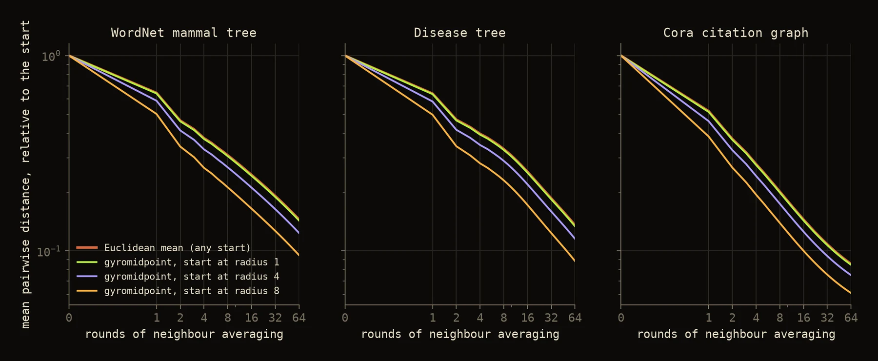
Table 3. Share of the starting spread left after rounds of averaging on the WordNet mammal tree. The Disease tree and Cora behave the same way.
| operator | 1 | 2 | 4 | 8 | 16 | 32 | 64 |
|---|---|---|---|---|---|---|---|
| Euclidean mean | 0.644 | 0.465 | 0.378 | 0.309 | 0.245 | 0.191 | 0.145 |
| gyromidpoint, start radius 1 | 0.640 | 0.461 | 0.374 | 0.305 | 0.242 | 0.189 | 0.143 |
| gyromidpoint, start radius 4 | 0.587 | 0.414 | 0.331 | 0.268 | 0.211 | 0.164 | 0.124 |
| gyromidpoint, start radius 8 | 0.502 | 0.342 | 0.266 | 0.212 | 0.165 | 0.127 | 0.095 |
Near the centre the two operators are the same, which is expected: the disk is flat to first order there. Further out the gyromidpoint contracts faster, at every round, on every graph. Hyperbolic averaging is still averaging.
10.2Trained networks
Averaging alone is not a network. So I trained four, all 32 real dimensions wide, for node classification:
- a Euclidean GCN with mean aggregation [21];
- a Poincare-ball network in the style of HGCN, which averages in the tangent space at the origin [5];
- the disks network of Equation 4;
- a control: the Euclidean GCN with the disks network's phase-keeping activation in place of ReLU.
Each was trained with 2, 4, 8, 16 and 32 message-passing layers, once with plain layers and once with a skip connection that mixes 10 % of the layer-0 state back in after every aggregation [19]. Two graphs: Cora, a citation network (2,708 nodes, public split, accuracy) [24], and the Disease tree of Chami et al. (1,044 nodes, 30/10/60 splits, F1) [5]. One configuration per graph, fixed in advance and identical for all models; five seeds; 400 training runs.
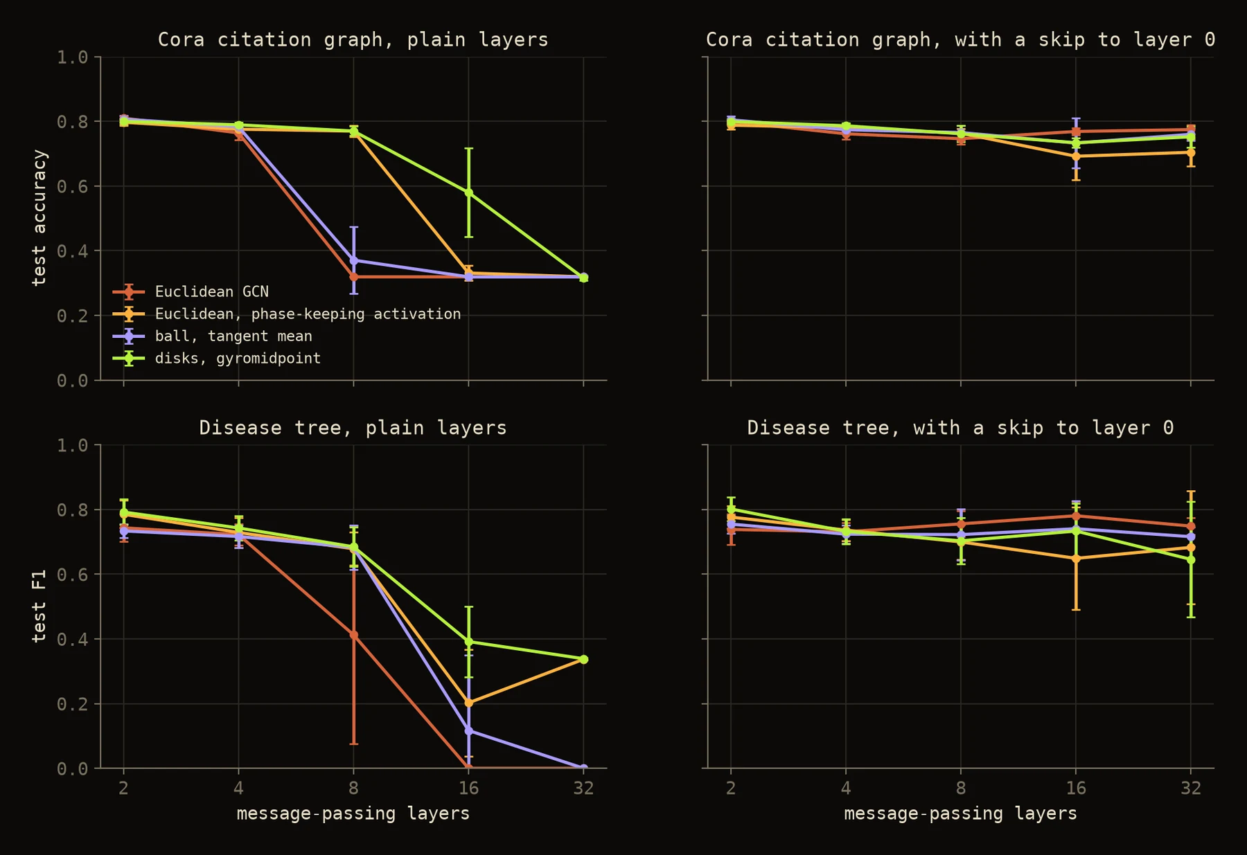
Table 4. Cora, test accuracy.
| network | layers | 2 | 4 | 8 | 16 | 32 |
|---|---|---|---|---|---|---|
| Euclidean GCN | plain | 0.810 ± 0.006 | 0.764 ± 0.021 | 0.319 ± 0.000 | 0.319 ± 0.000 | 0.319 ± 0.000 |
| Euclidean, phase-keeping activation | plain | 0.797 ± 0.010 | 0.775 ± 0.014 | 0.769 ± 0.017 | 0.331 ± 0.024 | 0.319 ± 0.000 |
| ball, tangent mean | plain | 0.807 ± 0.011 | 0.783 ± 0.010 | 0.371 ± 0.103 | 0.319 ± 0.000 | 0.319 ± 0.000 |
| disks, gyromidpoint | plain | 0.799 ± 0.009 | 0.789 ± 0.008 | 0.770 ± 0.014 | 0.580 ± 0.137 | 0.315 ± 0.008 |
| Euclidean GCN | with skip | 0.799 ± 0.005 | 0.761 ± 0.016 | 0.746 ± 0.017 | 0.768 ± 0.011 | 0.774 ± 0.015 |
| Euclidean, phase-keeping activation | with skip | 0.788 ± 0.013 | 0.780 ± 0.012 | 0.763 ± 0.015 | 0.692 ± 0.072 | 0.704 ± 0.043 |
| ball, tangent mean | with skip | 0.804 ± 0.011 | 0.774 ± 0.007 | 0.765 ± 0.022 | 0.733 ± 0.078 | 0.760 ± 0.019 |
| disks, gyromidpoint | with skip | 0.799 ± 0.009 | 0.786 ± 0.008 | 0.761 ± 0.025 | 0.733 ± 0.015 | 0.752 ± 0.032 |
Table 5. Disease tree, test F1.
| network | layers | 2 | 4 | 8 | 16 | 32 |
|---|---|---|---|---|---|---|
| Euclidean GCN | plain | 0.743 ± 0.042 | 0.722 ± 0.033 | 0.413 ± 0.337 | 0.000 ± 0.000 | 0.000 ± 0.000 |
| Euclidean, phase-keeping activation | plain | 0.785 ± 0.043 | 0.729 ± 0.046 | 0.678 ± 0.051 | 0.202 ± 0.165 | 0.337 ± 0.000 |
| ball, tangent mean | plain | 0.734 ± 0.022 | 0.716 ± 0.034 | 0.683 ± 0.069 | 0.117 ± 0.234 | 0.000 ± 0.000 |
| disks, gyromidpoint | plain | 0.792 ± 0.040 | 0.743 ± 0.038 | 0.685 ± 0.060 | 0.392 ± 0.109 | 0.339 ± 0.003 |
| Euclidean GCN | with skip | 0.738 ± 0.047 | 0.731 ± 0.028 | 0.756 ± 0.040 | 0.781 ± 0.044 | 0.749 ± 0.027 |
| Euclidean, phase-keeping activation | with skip | 0.776 ± 0.034 | 0.736 ± 0.033 | 0.700 ± 0.054 | 0.649 ± 0.159 | 0.683 ± 0.174 |
| ball, tangent mean | with skip | 0.755 ± 0.028 | 0.724 ± 0.028 | 0.722 ± 0.079 | 0.740 ± 0.085 | 0.716 ± 0.030 |
| disks, gyromidpoint | with skip | 0.801 ± 0.036 | 0.732 ± 0.039 | 0.703 ± 0.071 | 0.733 ± 0.086 | 0.646 ± 0.178 |
Four things stand out.
- The baselines are sane. At two layers every network reaches 0.80 to 0.81 on Cora, in line with the 81.5 % of the original GCN [21], and 0.73 to 0.80 on Disease, at or a little above what Chami et al. report for it (69.7 for GCN, 74.5 for HGCN) [5].
- Every plain network collapses. By 32 layers all four sit at the score of a constant prediction, on both graphs. The disks network is not an exception.
- The disks network does last longer, and the activation is why. At 8 layers on Cora the two ReLU networks have collapsed (0.32 and 0.37) while the disks network holds 0.770. But the Euclidean control with the same activation holds 0.769. The curvature adds nothing there. At 16 layers the disks network is ahead of the control (0.58 against 0.33) with a large spread across seeds, and at 32 both are gone.
- A skip connection fixes depth in every geometry. With it, all four networks train at 32 layers. On Cora the plain Euclidean GCN with a skip is the best of them at 16 and 32 layers (0.768 and 0.774), ahead of the disks network (0.733 and 0.752).
No network got reliably better with depth. The one apparent gain, the Euclidean GCN with a skip on Disease (0.738 at 2 layers, 0.781 at 16), is inside its spread across seeds. So the practical value of going deep is not shown here either.
The MAD of the last layer (Equation 6) tells the same story. All 87 runs that collapsed to a constant prediction have a MAD of 0.015 or less, whatever the geometry. Runs that still work have a median MAD of 0.89 on Cora and 0.57 on Disease. At four plain layers on Cora it is 0.79 for the Euclidean GCN, 0.86 for the ball and 0.91 for the disks.
Equation 6. Mean average distance (MAD) [18], on tangent vectors read as real vectors.
Correction
The first version reported MAD "often below 0.05 by layer 4" for Euclidean models and "stable at 0.62 or more" for this one, under the heading Empirical Proof. Those numbers did not come from an experiment. Measured, neither holds: no model is below 0.05 at four layers, and the disks model is at 0.01 by 32 plain layers. The formula there also used a hyperbolic inner product and norm that were never defined; the definition above is the standard one.
11Experiment 3: the whole pipeline on a tree
Experiments 1 and 2 test the pieces. This one runs them together: features go through the lift (Equation 1), then message passing over the training edges (Equation 4), and the network is trained with the contrastive loss (Equation 5) on the distance of its space (Equation 2). The data is the Disease link-prediction tree released with HGCN [5]: 2,665 nodes, 2,664 edges, 11 real features per node. 5 % of the edges are held out for validation and 10 % for testing, each with as many sampled non-edges, and a pair is scored by negative distance. The same four networks as before, 16 real dimensions wide, with 1, 2 and 4 layers; same loss and optimiser; five seeds.
Table 6. Link prediction on the Disease tree, test AUC, mean and standard deviation over 5 seeds.
| network | 1 layer | 2 layers | 4 layers |
|---|---|---|---|
| Euclidean GCN | 0.971 ± 0.008 | 0.750 ± 0.030 | 0.735 ± 0.019 |
| Euclidean, phase-keeping activation | 0.971 ± 0.008 | 0.787 ± 0.025 | 0.786 ± 0.032 |
| ball, tangent mean | 0.992 ± 0.003 | 0.989 ± 0.003 | 0.957 ± 0.016 |
| disks, gyromidpoint | 0.985 ± 0.006 | 0.962 ± 0.011 | 0.941 ± 0.014 |
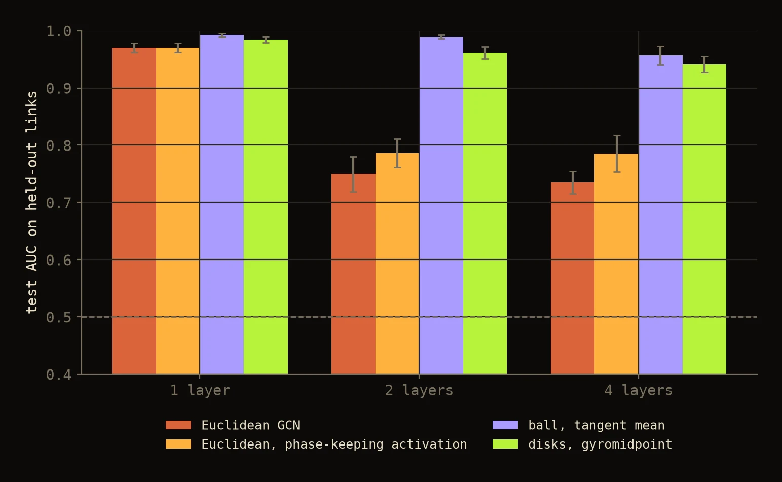
- Both hyperbolic pipelines work at every depth tried, between 0.94 and 0.99.
- The flat pipeline is close with one layer and far behind with more. With one layer it reaches 0.971, against 0.985 and 0.992, and it needs about ten times as many epochs to get there (about 5,600 against about 500). Left to train until it stopped improving by itself, it settles at 0.972. With two or four layers it falls to 0.74 to 0.79. I did not investigate why a second flat layer hurts this much on this tree.
- The standard ball is at least as good as the disks at every depth. The complex product structure is not what makes this work; the hyperbolic distance is.
Chami et al. report 64.7 for a Euclidean GCN and 90.8 for HGCN on their Disease link-prediction task [5]. Their decoder and loss are different from mine, so the numbers cannot be compared one to one. The direction is the same.
12What the experiments support
The first version ended with four claims that began "we solve". Here is each one against the measurements.
- Hierarchy pressure: supported, at low dimension. With 4 to 8 real dimensions the curved spaces keep a hierarchy that flat space loses (Table 1), and end to end on a tree they predict held-out links better (Table 6). It is a statement about a small dimension budget. With 32 dimensions flat space reconstructed the same hierarchy perfectly.
- Retrieval at high specificity: supported in the same narrow sense. Three quarters of the WordNet nodes are leaves, and at 8 dimensions a node's true relatives rank almost first (mean rank 1.05). That is one hierarchy of 1,170 nodes, not a retrieval benchmark.
- Relation fidelity: partly. Phase does carry a relation: which branch a node belongs to, recovered 99 % of the time from phases alone (Table 2). Typed relations such as "supports", "causes" and "depends on" were not tested here. The evidence that relation-as-rotation works is in RotatE and its hyperbolic successors [12, 13], not in this issue.
- Anti-collapse stability: not supported. The gyromidpoint contracts at least as fast as the mean (Table 3), every plain network collapses by 32 layers, and a skip connection is what fixes it, in every geometry (Tables 4 and 5).
And one finding the first version did not ask about. The product of complex disks never clearly beat the ordinary Poincare ball. It was ahead on reconstruction from 8 dimensions up, for a reason that may be optimisation, and behind on link prediction. The complex coordinates give a clean story about magnitude and phase. They have not yet earned their place over the simpler space.
13Limits
- Scale. Every graph here has between 1,044 and 2,708 nodes. One hierarchy for capacity, two graphs for depth, one tree for the pipeline.
- No retrieval benchmark. The motivation at the top is about memory for language models. Nothing here measures answer quality on text.
- No typed relations, as said above.
- Fixed curvature. Every hyperbolic space here has curvature −1. HGCN learns it per layer [5].
- A plain optimiser. Adam on tangent coordinates at the origin. Riemannian optimisers [1] might do better in two dimensions and on the ball.
- One configuration per dataset in Experiments 2 and 3, not tuned per model. Absolute numbers would move with tuning; I would expect the collapse of plain deep networks to stay.
- Depth never helped. On these tasks no model improved with depth by more than its spread across seeds, so the case for going deep was not made at all.
- Precision. Good hyperbolic embeddings sit very close to the rim and needed 64-bit floats here.
- Engineering cost. Hyperbolic operations, projection back into the disk and stability near the boundary all need care. Flat embeddings remain the right default for short-horizon retrieval. The case for this machinery is deep, branching, relation-sensitive data on a small dimension budget.
14Conclusion
The first version of this issue argued that better reasoning comes from better geometry, and offered numbers it had not measured. The measured version is narrower and I trust it more.
Curved space is worth dimensions. A hierarchy that flat space needs 32 dimensions to hold fits almost perfectly in 8 curved ones, and a pipeline built on hyperbolic distance predicts links on a tree that the flat one misses. That part of the proposal holds.
Curved space is not worth depth. Averaging in hyperbolic space is still averaging, and deep stacks of it collapse like any other until a skip connection holds them open. That part of the proposal was wrong.
And the complex-disk structure, the part that made this proposal its own, is so far a tidy idea with one confirmed property, phase carries branch, and no measured advantage over the ball.
Curved space bought capacity. It did not buy depth.
What survived testing
15Code
Everything above can be rerun. The geometry with its 18 tests, the three experiments, the result files and the figure scripts are in github.com/nsquaredzz/escaping-flatland.
References
- Nickel, M., and Kiela, D. (2017). Poincare Embeddings for Learning Hierarchical Representations. NeurIPS.
- Sarkar, R. (2011). Low Distortion Delaunay Embedding of Trees in Hyperbolic Plane. Graph Drawing.
- Sala, F., De Sa, C., Gu, A., and Re, C. (2018). Representation Tradeoffs for Hyperbolic Embeddings. ICML.
- Ganea, O., Becigneul, G., and Hofmann, T. (2018). Hyperbolic Neural Networks. NeurIPS.
- Chami, I., Ying, R., Re, C., and Leskovec, J. (2019). Hyperbolic Graph Convolutional Neural Networks. NeurIPS.
- Liu, Q., Nickel, M., and Kiela, D. (2019). Hyperbolic Graph Neural Networks. NeurIPS.
- Gu, A., Sala, F., Gunel, B., and Re, C. (2019). Learning Mixed-Curvature Representations in Product Spaces. ICLR.
- Ungar, A. A. (2008). Analytic Hyperbolic Geometry and Albert Einstein's Special Theory of Relativity. World Scientific.
- Gulcehre, C., et al. (2019). Hyperbolic Attention Networks. ICLR.
- Shimizu, R., Mukuta, Y., and Harada, T. (2021). Hyperbolic Neural Networks++. ICLR.
- Xiao, H., Jiang, C., Song, Y., Zhang, J., and Xiong, J. (2021). Unit Ball Model for Embedding Hierarchical Structures in the Complex Hyperbolic Space. arXiv:2105.03966.
- Sun, Z., Deng, Z.-H., Nie, J.-Y., and Tang, J. (2019). RotatE: Knowledge Graph Embedding by Relational Rotation in Complex Space. ICLR.
- Chami, I., Wolf, A., Juan, D.-C., Sala, F., Ravi, S., and Re, C. (2020). Low-Dimensional Hyperbolic Knowledge Graph Embeddings. ACL.
- Zhang, X., He, Y., Brugnone, N., Perlmutter, M., and Hirn, M. (2021). MagNet: A Neural Network for Directed Graphs. NeurIPS.
- Chen, T., Kornblith, S., Norouzi, M., and Hinton, G. (2020). A Simple Framework for Contrastive Learning of Visual Representations. ICML.
- Ge, S., Mishra, S., Kornblith, S., Li, C.-L., and Jacobs, D. (2023). Hyperbolic Contrastive Learning for Visual Representations beyond Objects. CVPR.
- Li, Q., Han, Z., and Wu, X.-M. (2018). Deeper Insights into Graph Convolutional Networks for Semi-Supervised Learning. AAAI.
- Chen, D., Lin, Y., Li, W., Li, P., Zhou, J., and Sun, X. (2020). Measuring and Relieving the Over-smoothing Problem for Graph Neural Networks from the Topological View. AAAI.
- Chen, M., Wei, Z., Huang, Z., Ding, B., and Li, Y. (2020). Simple and Deep Graph Convolutional Networks. ICML.
- Liu, J., Yi, X., and Huang, X. (2024). DeepHGCN: Toward Deeper Hyperbolic Graph Convolutional Networks. IEEE Transactions on Artificial Intelligence.
- Kipf, T. N., and Welling, M. (2017). Semi-Supervised Classification with Graph Convolutional Networks. ICLR.
- Arjovsky, M., Shah, A., and Bengio, Y. (2016). Unitary Evolution Recurrent Neural Networks. ICML.
- Miller, G. A. (1995). WordNet: A Lexical Database for English. Communications of the ACM.
- Sen, P., et al. (2008). Collective Classification in Network Data. AI Magazine.
First published as issue #002 of The Multiverse of Intelligence. This is the revised and tested version.